When I learned that the newly discovered B₈₀ boron buckyball can be viewed as a modified C₆₀ buckminsterfullerene, I wondered whether it could be reconstructed directly from the built-in Buckminsterfullerene graph. It turns out that a few graph operations go a long way: by adding a vertex to each hexagonal face and connecting it to the surrounding cage, the familiar C₆₀ structure transforms into a model of the B₈₀ boron fullerene. This post walks through the construction and explores the resulting graph and geometry. CITATION (original article): Hyun Wook Choi, et al., Chem. Sci., 2026, Advance Article. https://doi.org/10.1039/D6SC02674E
Import the base graph:
In[]:=
c60=GraphData["Buckminsterfullerene"]
Out[]=
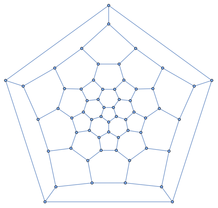
Find the coordinates of the vertices in the graph:
In[]:=
coordDict=AssociationThread[VertexList[c60]->GraphEmbedding[c60]];
Placing an additional boron atom at the center of each hexagonal face of the C₆₀ cage:
In[]:=
f1[v_,l_List]:=v#&/@lf2[v_,l_List]:=v->RegionCentroid[Polygon[coordDict/@l]]
In[]:=
hexFaces=Select[PlanarFaceList[c60],Length[#]==6&];
The planar embedding of Boron 80 buckyball:
In[]:=
b80bucky=With[{vtxSet2=Range[61,61+Length[hexFaces]-1]},{additionalEdges=MapThread[f1,{vtxSet2,hexFaces}]//Flatten,additionalCoord=MapThread[f2,{vtxSet2,hexFaces}]},Graph[EdgeList[c60]~Join~additionalEdges,VertexCoordinates->Join[Normal@coordDict,additionalCoord]]]
Out[]=
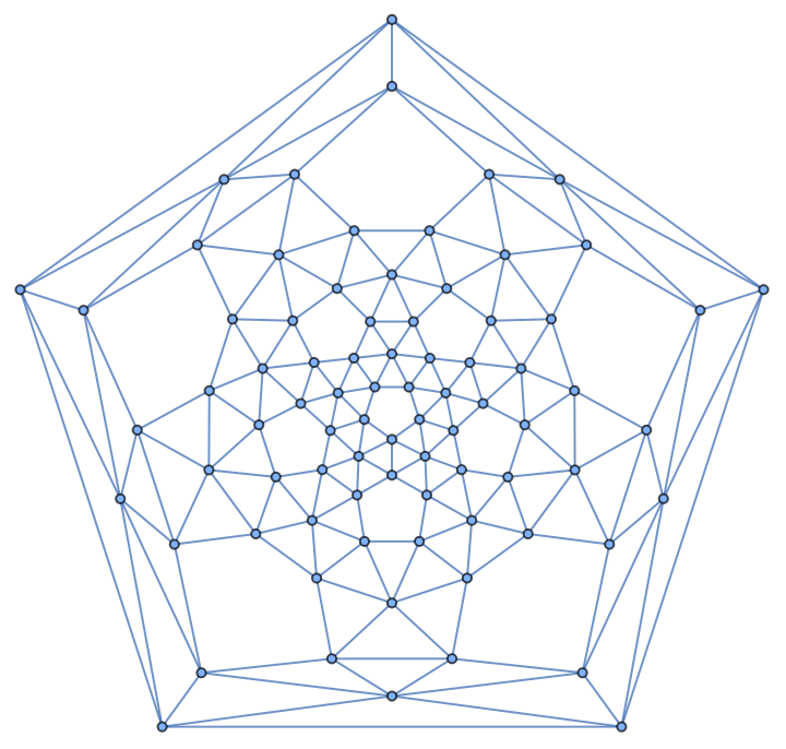
Create the 3D spherical embedding of the graph:
In[]:=
b80bucky3D=Graph3D[b80bucky//EdgeList,GraphLayout->"SphericalEmbedding"]
Out[]=

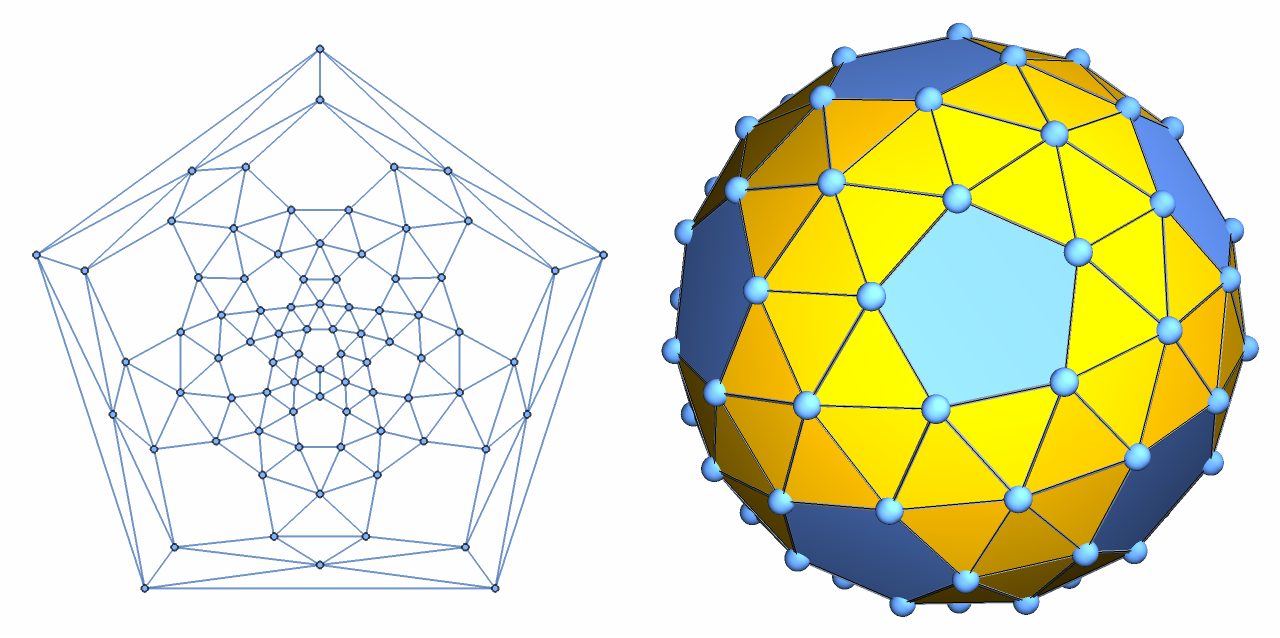
Highlight the faces of the structure:
In[]:=
Module[{db,coordsDict3},db=GroupBy[PlanarFaceList[b80bucky],Length];coordsDict3=AssociationThread[(b80bucky3D//VertexList)->GraphEmbedding[b80bucky3D]];{facePoly3,facePoly5}=(Polygon/@Map[coordsDict3,#,{2}])&/@{db[3],db[5]}];
Visualize the planar graph and its three-dimensional embedding side by side:
In[]:=
GraphicsRow[{b80bucky,Show[b80bucky3D,Graphics3D[{{StandardYellow,facePoly3},{StandardBlue,facePoly5}},Boxed->False]]}]
Out[]=
A few additional explorations of the graph’s properties
A few additional explorations of the graph’s properties
◼
The Boron 80 buckyball is not regular.
In[]:=
ResourceFunction["RegularGraphQ"][b80bucky]
Out[]=
False
◼
Find the adjacency matrix and its spectrum.
In[]:=
ord=Ordering[VertexList[b80bucky]];am=AdjacencyMatrix[b80bucky][[ord,ord]];ArrayPlot[am,ColorRules->{0->Purple,1->StandardYellow}]
Out[]=
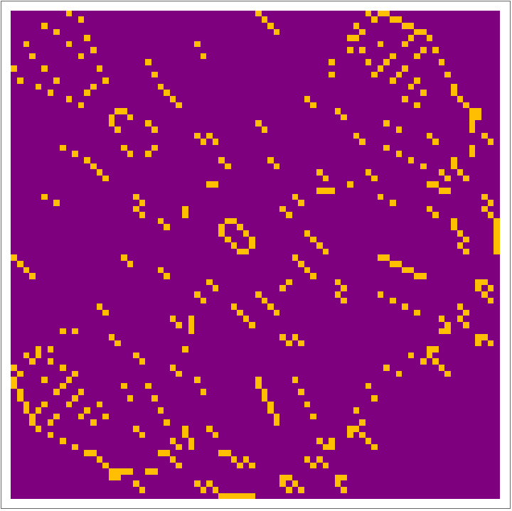
All eigenvalues are real because the matrix is symmetric:
ListPlotSortBy[Chop@Eigenvalues[N@am],Abs],
Out[]=
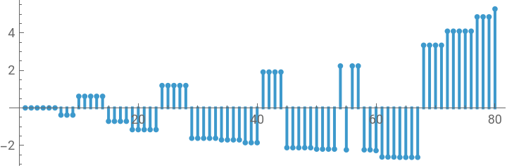
The corresponding characteristic polynomial and its graph on complex plane:
In[]:=
cp=CharacteristicPolynomial[am,x.]//Factor
◼
Find a Hamiltonian path on the graph, a continuous route that visits every vertex exactly once without revisiting any vertex.
◼
Find a perfect matching on the graph, which is a set of edges such that every vertex is connected to exactly one selected edge.
◼
Find the dual planar graph, where each face of the planar embedding becomes a vertex and adjacent faces are connected by an edge.
◼
Create a similar pair of the planar and spherical embedding for the dual graph.
◼
Find a Hamiltonian path on the dual graph.
◼
Find the adjacency matrix, the spectrum and characteristic polynomial of the dual graph.
Reference
Reference
◼
Introducing boron buckyballs, https://doi.org/10.47287/cen.485651.newsarticle, Chemical & Engineering News, ISSN 0009-2347, Copyright © 2026 American Chemical Society
CITE THIS NOTEBOOK
CITE THIS NOTEBOOK
Recreating the Boron 80 buckyball with graph functions
by Shenghui Yang
Wolfram Community, STAFF PICKS, June 7, 2026
https://community.wolfram.com/groups/-/m/t/3729403
by Shenghui Yang
Wolfram Community, STAFF PICKS, June 7, 2026
https://community.wolfram.com/groups/-/m/t/3729403