In this short computational essay, I explored various wave packets constructed from special functions, focusing on Airy, Bessel, and Gaussian waveforms and their combinations. Similar studies have been conducted in optics, as evidenced by the references provided. Here, I extended this exploration to the Schrödinger equation. The Airy-Bessel-Gauss case is usually called as the light bullet in optics literature.
Non-spreading Airy wave packet
Non-spreading Airy wave packet
In[]:=
ClearAll[airyWP]airyWP[x_,t_]:=AiryAi[x-t^2/4]Exp[t/2(x-t^2/6)]
Check it satisfies the dynamical equation (paraxial equation or same as Schrodinger equation):
In[]:=
D[airyWP[x,t],t]==-1/2D[airyWP[x,t],{x,2}]//FullSimplify
Out[]=
True
Visualize the result:
In[]:=
Manipulate[Plot[Abs[AiryAi[x-t^2/4]Exp[t/2(x-t^2/6)]]^2,{x,-30,30},PlotPoints->50,PlotRange->{0,.5},AxesLabel->{"Time","Abs[ψ]"}],{t,0,10},SaveDefinitions->True]
Out[]=


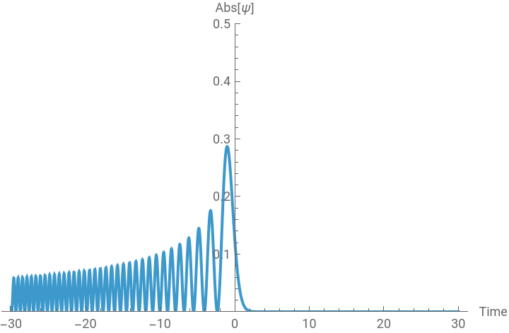
Note it propagates without changing its form and no spreading.
Airy beam
Airy beam
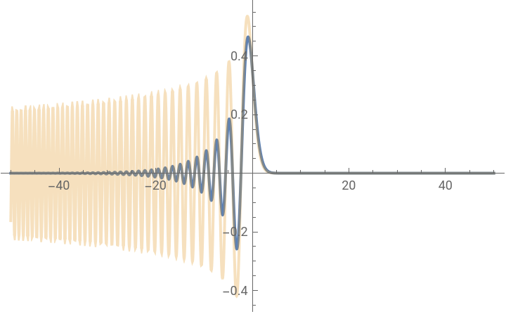
The fact that the Airy function is not square-integrable over all of means it cannot represent a normalizable wave function for the Schrödinger equation in quantum mechanics. This can be resolved by adding an exponential term:
In[]:=
Plot{AiryAi[x]Exp[ax]/.a->.15,AiryAi[x]},{x,-50,50},PlotRange->All,PlotStyle->{Automatic,Opacity[.3]},PlotLegends->{"Airy with exponential term (Ai(x))","Airy"}
0.15x
Out[]=


Accordingly, the time evolution of above wave function is given by:
In[]:=
ClearAll[airyBeam];airyBeam[z_,t_]:=Expaz-Expt-+AiryAiz+at-
a
2
t
2
2
a
2
3
t
12
zt
2
2
t
4
In[]:=
airyBeam[z,t]//TraditionalForm
Out[]//TraditionalForm=
expt-+-+azAi-+at+z
2
a
2
3
t
12
tz
2
a
2
t
2
2
t
4
Check it satisfies the equation :
+(z,t)=0
∂(z,t)
ψ
Ai
∂t
1
2
2
∂
ψ
Ai
∂
2
z
In[]:=
FullSimplifyD[airyBeam[z,t],t]+D[airyBeam[z,t],{z,2}]==0,Assumptions->{a,t}∈Reals
1
2
Out[]=
True
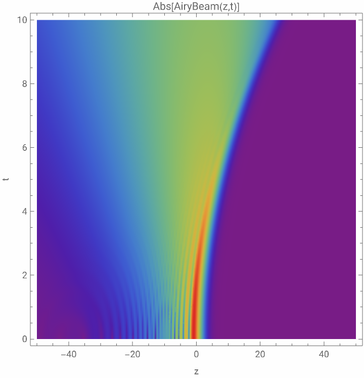
Visualize time evolution:
In[]:=
DensityPlot[Abs[airyBeam[z,t]/.{a->.15}],{z,-50,50},{t,0,10},PlotRange->All,ColorFunction->(ColorData["Rainbow"][Sqrt[#]]&),PlotPoints->200,FrameLabel->{"z","t"},PlotLegends->Automatic,PlotLabel->"Abs[AiryBeam(z,t)]"]
Out[]=

In[]:=
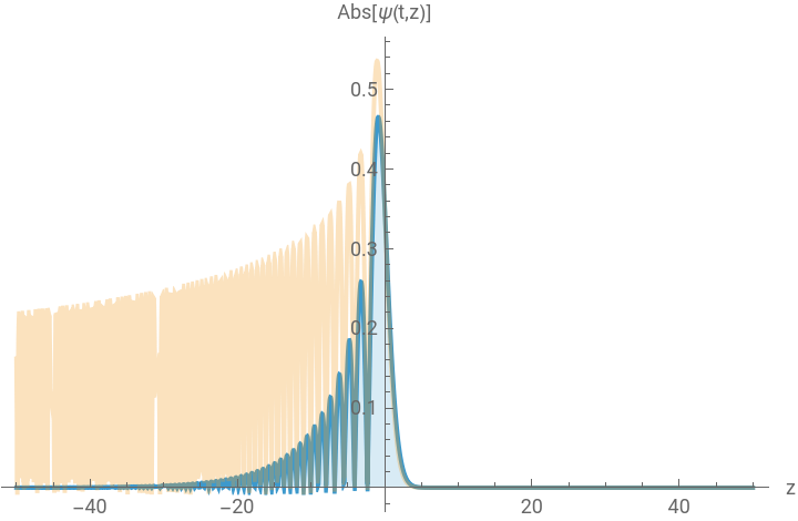
Manipulate[Plot[{Abs[airyBeam[z,t]/.a->.15],Abs[airyBeam[z,t]/.a->0]},{z,-50,50},PlotRange->All,PlotStyle->{Automatic,Directive[Opacity[.3]]},Filling->1->Bottom,PlotLegends->{"Airy beam (a≠0)","Nonspreading Airy beam (a=0)"},AxesLabel->{"z","Abs[ψ(t,z)]"}],{t,0,10,.1},SaveDefinitions->True]
Out[]=


Bessel-Gauss beam
Bessel-Gauss beam
A Bessel-Gauss function as initial field: (x,y,0)=(rβ) with
ψ
BG
-
2
r
2
w0
J
0
r=+
2
x
2
y
In[]:=
Plot3DBesselJ0,(rβ) with β=3 and w0=7"
-
x^2+y^2
2
w0
x^2+y^2
β/.{β->3,w0->7},{x,-15,15},{y,-15,15},ColorFunction->"Rainbow",PlotRange->All,PlotPoints->200,PlotLegends->Automatic,PlotLabel->"-
2
r
2
w0
J
0
Out[]=
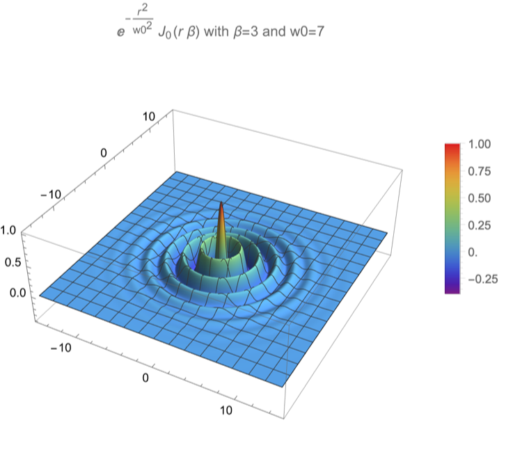
To solve above integral, first some change of variables:
Try to solve the original Fresnel integral by plugging above result:
Since it does not work (or at least, I was not able to coach Mathematica to do the above integral), I searched the literature for similar results.
To solve above equation, I looked up into this book (Weber’s 2nd exponential integral):
Watson, G. N. (1966). A treatise on the theory of Bessel functions (2nd ed.). Cambridge University Press. (p. 395, Eq. 1)
Watson, G. N. (1966). A treatise on the theory of Bessel functions (2nd ed.). Cambridge University Press. (p. 395, Eq. 1)
Find p:
which is fully satisfied. Therefore, one finds:
Define Bessel-Gaussian beam:
Visualize:
Airy-Bessel-Gauss
Airy-Bessel-Gauss
Combine Airy with Bessel-Gauss:
It traditional form:
Check that Airy-Bessel-Gauss beam satisfies Schrodinger equation:
Create density plot for different times (this step takes a long time):
Export them as GIF:
Create cross-sections (this step is time-consuming):
Animate them:
Initially, the Bessel component dominates along the x-axis in the visualizations above, but the Gaussian component becomes increasingly significant over time. Meanwhile, the evolution along the x-axis in these visualizations is governed by the Airy beam.
Export as a GIF
CITE THIS NOTEBOOK
CITE THIS NOTEBOOK
Quantum bullet: Airy, Bessel and Gauss
by Mohammad Bahrami
Wolfram Community, STAFF PICKS, December 17, 2024
https://community.wolfram.com/groups/-/m/t/3341082
by Mohammad Bahrami
Wolfram Community, STAFF PICKS, December 17, 2024
https://community.wolfram.com/groups/-/m/t/3341082