Imagine a tunnel drilled straight through the center of the Earth, connecting one side of the planet to the other. What would happen if an object were released to fall freely inside this passage? In this computational essay, not merely as coding, but as a comprehensive project that integrates physics, mathematics, and programming, we will explore the problem both physically and mathematically. My primary audience is students, and the purpose is to present physics (e.g., simple harmonic motion) and mathematics (e.g., differential equations) in an engaging way by leveraging the capabilities of Wolfram Language (coding, visualizations, animations). Using the Wolfram Language, with its powerful symbolic engine and dynamic visualization tools, we can clarify concepts, simulate motion, and bring abstract ideas to life. All presented in an aesthetic, story-driven way that shows mathematics as both science and art.
1 Model Setup and Assumptions
1 Model Setup and Assumptions
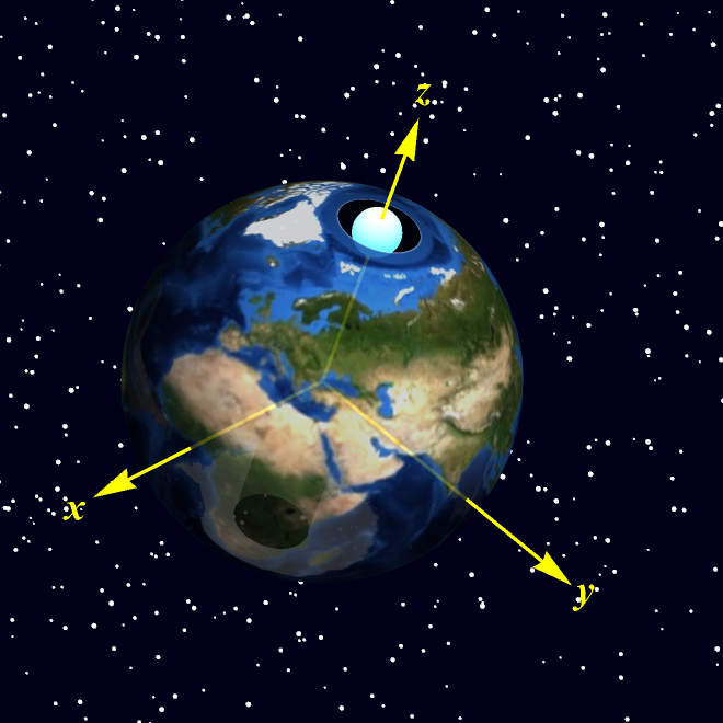
The following assumptions provide an abstraction of the idea, and consequently, a simplification of the analysis. We assume the Earth is treated as a perfect sphere with uniform density. Only Newtonian gravity is considered, while the effects of rotation, pressure, and temperature are ignored. The tunnel is assumed to be already constructed, completely evacuated, and free of friction along its walls. Without loss of generality, the tunnel passes straight through the Earth’s center from pole to pole, and it is assumed to be narrow enough to neglect any change in the mass distribution. Together with any other idealizations naturally consistent with this setup, these assumptions give us full license for a clean theoretical treatment. For the mathematical framework, a Cartesian coordinate system is placed with its origin at the Earth’s center and the -axis aligned with the tunnel. The falling body is treated as a point mass starting its free fall from the North Pole, and the sketch is regarded as schematic rather than to scale (Fig. 1).
z
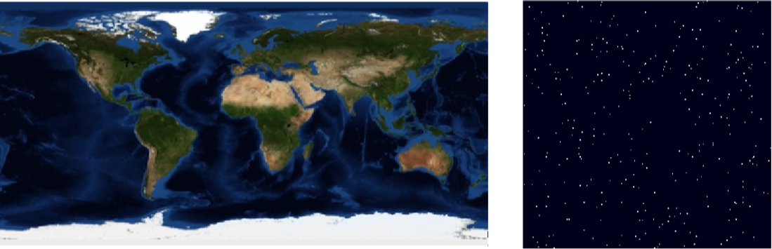
Generate a world map texture and create a starry background for the scene:
worldTexture=GeoGraphics["World",GeoBackground"Satellite"];SeedRandom[2025];skyTexture=GraphicsStyle,Table[Style[Point[RandomReal[{-1.5,1.5},2]],White,PointSize[RandomReal[{0.005,0.002}]]],1000],;Row[{Image[worldTexture,ImageSize->500],Image[skyTexture,ImageSize->250]}," "]
Out[]=
Construct the 3D scene with Earth, axes, tunnel, and the falling body, then render the figure with a starry background:
Module{radius,amp,theta,viewPoint,slant,axes,body,earth,tunnel,wall,fig1},radius=1;amp=radius-0.06;theta=π2;viewPoint={0,-5,0};slant=RotationTransform[23°,viewPoint][{0,0,1}];axes=Graphics3D,Boxed->False;body=Graphics3D[Style[Sphere[{0,0,ampSin[theta]},0.12],Glow[Cyan]]];earth=ParametricPlot3Dradius{Cos[u+theta]Cos[v],Sin[u+theta]Cos[v],Sin[v]},{u,0,2π},{v,-π/2.3,π/2.3},;tunnel=ParametricPlot3D{0.2Cos[ϕ],0.2Sin[ϕ],0.97z},{ϕ,0,2π},{z,-1,1},;wall=ParametricPlot3D{0.2Cos[ϕ],0.2Sin[ϕ],0.97z},{ϕ,0,π},{z,-1,1},;fig1=GraphicsInset[skyTexture,{0,0},Center,Scaled[1]],InsetShow{earth,body,axes,tunnel},,{0,0},Center,Scaled[1],ImageSize->600;Labeled[ImageCrop[fig1,{660,660}],Style["Fig. 1: Earth with coordinate axes, a central tunnel, and the falling body.",FontFamily->"Times"]]
Out[]=
Fig. 1: Earth with coordinate axes, a central tunnel, and the falling body. |
2 Newton’s Second Law
2 Newton’s Second Law
In this part, we express Newton’s second law in vector form. Let (t)x(t)+y(t)+z(t) be the position vector of a test particle of mass . The motion of the particle is governed by Newton’s second law, (t)m(t), where (t) is the total force acting on the particle and (t) denotes its acceleration, with the double dot indicating the second derivative with respect to time. This provides the general mechanical framework before specifying the gravitational force, which we will derive next using two different methods. In the following code cells, we adhere to the same mathematical notation as in the text, incorporating vector symbols to maintain a direct connection between the mathematics and the code.
r
i
j
k
m
F
Newton
¨
r
F
Newton
¨
r
Define the position vector of the particle as a function of time:
In[]:=
r
Define the force according to Newton’s second law (where the double dash in the code denotes the second derivative with respect to time):
In[]:=
forceNewton
r
forceNewton
Out[]=
{m[t],m[t],m[t]}
′′
x
′′
y
′′
z
3 Gravitational Force from Earth’s Density
3 Gravitational Force from Earth’s Density
Building on the previous framework, the first method derives the gravitational force directly from the assumption of a uniform-density Earth. The enclosed mass within a sphere of radius (t) is given by:
r
M(t)πr(t)ρ
4
3
3
where is the enclosed mass at time , and is the magnitude of the position vector at time . The gravitational force (t) on a test particle of mass is then obtained from Newton’s law of gravitation:
M(t)
t
r(t)||(t)||
r
x+y+z
2
(t)
2
(t)
2
(t)
t
F
Density
m
F
Density
M(t)m
2
r(t)
r
Here, is the gravitational constant, and (t)r(t) is the unit vector in the radial direction. The force is always directed inward, opposite to the position vector, pointing toward the center of the Earth. The negative sign in Newton’s law of gravitation accounts for this reversal of direction. According to our assumptions, since the particle begins at the Earth’s surface, the initial enclosed mass is ℳ (the total mass of the Earth), and the initial position magnitude is ℛ (the Earth’s radius). Under the uniform-density assumption, the Earth’s density is therefore expressed as:
r
r
M(0)
r(0)
ρ=π
ℳ
4
3
3
ℛ
Define the initial position magnitude and the general expression for :
r(0)
r(t)
In[]:=
r[0]=ℛ;r[t_]:=++
2
x[t]
2
y[t]
2
z[t]
Define the initial enclosed mass and the general formula for :
M(0)
M(t)
In[]:=
M[0]=ℳ;M[t_]:=πρ
4
3
3
r[t]
Define the gravitational force vector (t) and substitute the uniform-density relation:
F
Density
In[]:=
forceDensity
M[t]m
2
r[t]
r
r[t]
ℳ
4
3
3
ℛ
forceDensity
Out[]=
-,-,-
mℳx[t]
3
ℛ
mℳy[t]
3
ℛ
mℳz[t]
3
ℛ
4 Gravitational Force from Earth’s Potential
4 Gravitational Force from Earth’s Potential
The second approach starts from the scalar gravitational potential. The potential of a spherical body (the Earth in this case) is expressed piecewise [3]:
Φ(t)=
|
The gravitational acceleration (t) is obtained from the negative gradient of the scalar potential:
g
g
∂Φ
∂x
i
∂Φ
∂y
j
∂Φ
∂z
k
Here, denotes the gradient operator, and represents partial differentiation with respect to the corresponding spatial coordinates. For a point mass falling inside the tunnel through the Earth, we restrict to ℛ, and denote the result as (t). Multiplying by the mass then yields the gravitational force vector (t) acting on the particle.
∇
∂
r(t)≤
g
Interior
m
F
Potential
Define the scalar potential:
In[]:=
Φ[t_]:=
|
Define the gravitational acceleration (t) as the negative gradient of the potential :
g
Φ(t)
In[]:=
g
∇
{x[t],y[t],z[t]}
Restrict the acceleration to the interior of the Earth:
In[]:=
gInterior
g
Define the force as times the interior acceleration (t) :
F
Potential
m
g
Interior
In[]:=
forcePotential
gInterior
forcePotential
Out[]=
-,-,-
mℳx[t]
3
ℛ
mℳy[t]
3
ℛ
mℳz[t]
3
ℛ
5 Equation of Motion
5 Equation of Motion
Finally, we compare the two approaches. Both the density method and the potential method yield the same expression for the gravitational force inside the Earth.
Compare the force expressions derived from density and potential:
Set the initial conditions:
Solve the differential equation with the initial conditions:
This result demonstrates that the motion of the particle is simple harmonic, oscillating through the tunnel with amplitude ℛ and angular frequency ω.
6 Kinematics of the Gravity Train
6 Kinematics of the Gravity Train
Now that the mathematical groundwork has been completed, it is time to harvest the results. We can directly observe the kinematic equations for position, speed, and acceleration of the motion.
Derive position, speed, and acceleration from the analytic solution by successive differentiation:
We now substitute the numerical values of Earth’s constants to obtain explicit time-dependent expressions for position, speed, and acceleration. Finally, the oscillation period is evaluated and divided by 60 to express the result in minutes.
Substitute Earth’s constants for numerical evaluation:
Evaluate the position, speed, and acceleration:
Convert the period into minutes:
The result is remarkable: the full oscillation period is about 84 minutes. This means a gravity train would carry you from the North Pole to the South Pole in just half of that time, around 42 minutes, making it an incredibly fast journey across the planet.
7 Visualizations
7 Visualizations
We now plot the kinematic functions—position, velocity, and acceleration—over one full oscillation period, with time expressed in units of the period.
Plot the position, speed, and acceleration as functions of time over one period:
To visualize the gravity train in a more compelling way, we animate the motion of the particle inside a rotating Earth. Although the influence of Earth’s rotation was neglected in the analytical model, here it is included purely for aesthetic realism. In particular, when the tunnel is aligned with the Earth’s rotation axis, rotational effects essentially vanish. The animation respects the true ratio between Earth’s spin and the oscillation of the train: 17 oscillation periods of the particle correspond almost exactly to one full day of Earth’s rotation, giving a visually realistic 24-hour cycle.
Generate animation frames showing Earth’s rotation, the tunnel, and the oscillating body against a starry background:
Play the sequence of frames as an interactive animation:
References
References
[1] Wolfram Science World: Sphere Gravitational Potential Energy [Online]. Accessed: October 4, 2025.
[4] Andrew J. Simoson. 2018. Falling down a Hole through the Earth. Mathematics Magazine, 77(3), 171–189. DOI: 10.1080/0025570X .2004.11953248.
[5] Thomas Concannon and Gerardo Giordano. 2016. Gravity Tunnel Drag. arXiv preprint: arXiv:1606.01852.
[7] Alexander R. Klotz. 2013. The Gravity Tunnel in a Non-Uniform Earth. arXiv preprint: arXiv:1308.1342.
CITE THIS NOTEBOOK
CITE THIS NOTEBOOK
Gravity train dynamics in a tunnel through the Earth
by Akram Masoud
Wolfram Community, STAFF PICKS, October 6, 2025
https://community.wolfram.com/groups/-/m/t/3555794
by Akram Masoud
Wolfram Community, STAFF PICKS, October 6, 2025
https://community.wolfram.com/groups/-/m/t/3555794