TheLimitCycleInPredatorPreyModels::usage="A model is:x'[t] = r x[t]1 - - y[t]y'[t] = - c y[t] + d y[t]where:x = number of prey, y = number of predators predadores. The others are positive constants.The term R = represents the number of prey devoured per unit of time.The constant a can be interpreted as the maximum number of prey that can be devoured by a predator per unit of time.A particular case is resolved in which χ[0] = {20, 3}.Referencia: Zill, D.G. and Cullen, M.R. Differential Equations with Boundary-Value Problems. Ed. Brooks/Cole: pp.417-419, 1997; Personal.";
x[t]
K
ax[t]
b+x[t]
ax[t]
b+x[t]
ax[t]
b+x[t]
In[]:=
diffeqs[{x0_,y0_}]:=x'[t]==1.5x[t]1--y[t],y'[t]==-4y[t]+2y[t],x[0]==x0,y[0]==y0;endTime=17;initPt={19,3};soln=Flatten[NDSolve[diffeqs[initPt],{x,y},{t,0,endTime}]]
x[t]
45
5x[t]
18+x[t]
5x[t]
18+x[t]
Out[]=
xInterpolatingFunction,yInterpolatingFunction


In[]:=
s1=ParametricPlot[Evaluate[{y[t],x[t]}/.soln],{t,0,17}]
Out[]=
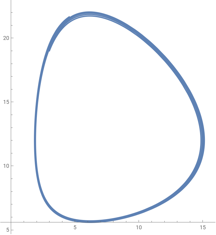
In[]:=
diffeqs[{x0_,y0_}]:=x'[t]==1.5x[t]1--y[t],y'[t]==-4y[t]+2y[t],x[0]==x0,y[0]==y0;endTime=17;initPt={10,15};soln=Flatten[NDSolve[diffeqs[initPt],{x,y},{t,0,endTime}]]
x[t]
45
5x[t]
18+x[t]
5x[t]
18+x[t]
Out[]=
xInterpolatingFunction,yInterpolatingFunction


In[]:=
s2=ParametricPlot[Evaluate[{y[t],x[t]}/.soln],{t,0,17}]
Out[]=
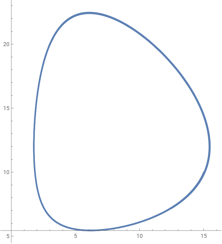
In[]:=
diffeqs[{x0_,y0_}]:=x'[t]==1.5x[t]1--y[t],y'[t]==-4y[t]+2y[t],x[0]==x0,y[0]==y0;endTime=17;initPt={14,8};soln=Flatten[NDSolve[diffeqs[initPt],{x,y},{t,0,endTime}]]
x[t]
45
5x[t]
18+x[t]
5x[t]
18+x[t]
Out[]=
xInterpolatingFunction,yInterpolatingFunction


In[]:=
s3=ParametricPlot[Evaluate[{y[t],x[t]}/.soln],{t,0,17}]
Out[]=
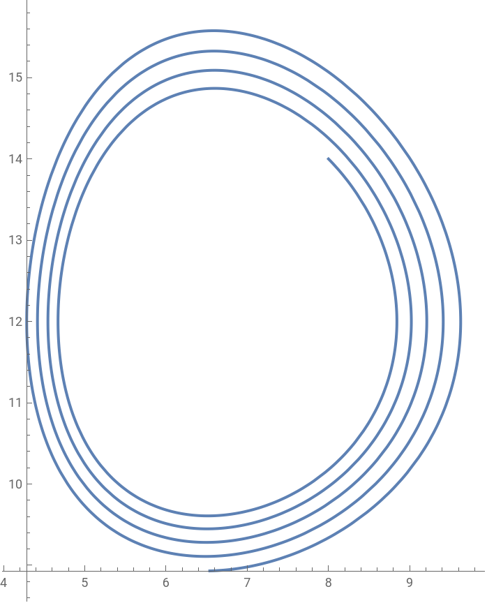
In[]:=
diffeqs[{x0_,y0_}]:=x'[t]==1.5x[t]1--y[t],y'[t]==-4y[t]+2y[t],x[0]==x0,y[0]==y0;endTime=17;initPt={12,6.6};soln=Flatten[NDSolve[diffeqs[initPt],{x,y},{t,0,endTime}]]
x[t]
45
5x[t]
18+x[t]
5x[t]
18+x[t]
Out[]=
xInterpolatingFunction,yInterpolatingFunction


In[]:=
s4=ParametricPlot[Evaluate[{y[t],x[t]}/.soln],{t,0,17}]
Out[]=
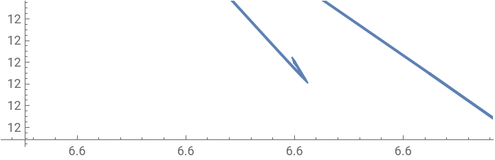
In[]:=
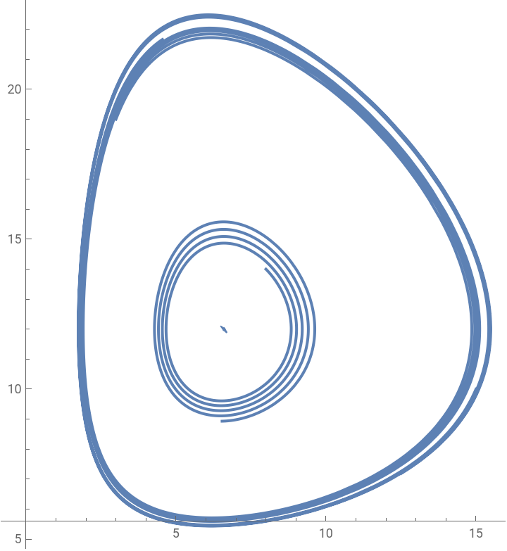
Show[s1,s2,s3,s4]
Out[]=