Sailing is a very complex sport deeply based in physics also requiring a lot of tactics to analyze the best path to get around the course in a race. In my project, I created a wind tunnel with the Lattice Boltzmann method to analyze how much lift will be generated for different combinations of wind speed, boat angle and sail angle. I then applied the results to a generated wind vector field to optimize the path between one point and another.
Introduction
Introduction
Sailing straight into the wind is obviously impossible, so in order to sail upwind, I must sail at around 45 degree angles off the wind direction to slowly zigzag my way up the course. By heading a lower angle (larger angle from the wind direction), the boat will increase in speed but increase in distance sailed, and in sailing one of the challenges is to be able to constantly find the perfect balance between speed and distance to sail. Another integral part of sailing is to analyze the wind and look for gusts (patches of stronger wind) and shifts (wind direction changes). In order to sail around the course quickly, I must sail to the gusts as soon as possible as well as choose the correct side to sail to: right when the wind shifts right and left when the wind shifts left.
Designing the sails
Designing the sails
I used two manipulate functions and Bezier curves to manually adjust the sail-shape while making sure the arc-length stays constant and accurate to the real life measurements.
Making the jib
Making the jib
The jib is the smaller of the two sails and is positioned in front of the mainsail to redirect the flow of wind into the mainsail, therefore the jib has an open leach so air can flow out of the jib into the main sail.
The arc length of the jib should be roughly 169 cm and the difference between the x value of the two endpoints should be 163 cm.
◼
jmat is the rotation matrix for the jib
◼
jpts are the points used for the bezier curve
◼
ja is the manipulated variable to adjust the depth of the sail near the front
◼
jb is the manipulated variable for how open the sail is at the back
◼
jAOA is the angle the jib will be facing in relation to the boat angle
I chose 37.5 for ja and 30 for jb.
In[]:=
Clear[jmat,jpts,ja,jb,jt,jAOA];Manipulate[jpts={{0,0},{50,ja},{163,jb}};jmat={{Cos[(jAOA) Degree],-Sin[(jAOA) Degree]},{Sin[(jAOA) Degree],Cos[(jAOA) Degree]}};jf=BezierFunction[jpts];ParametricPlot[jmat.{jf[jt][[1]],jf[jt][[2]]},{jt,0,1},AspectRatio->Automatic,ImageSize->Medium,PlotRange->{{0,200},{-45,40}}],{{ja,0.9},0.1,50},{{jb,0.9},0.1,50},{{jAOA,0,"Angle of Attack"},-45,45},Dynamic[StringJoin["Arc length: ",ToString[NIntegrate[Sqrt[Power[D[2(1−jt)jt*50+(jt^2)*163,jt],2]+Power[D[2(1−jt)jt*ja+(jt^2)*jb,jt],2]],{jt,0,1}]]," cm"]],SaveDefinitions->True]
Out[]=


Making the mainsail
Making the mainsail
The mainsail is much larger than the jib but has a closed leach in order to provide more lift.
The arc length of the main should be approximately 199.5 cm and the distance between the two endpoints should be 194 cm .
◼
mat is the rotation matrix for the main sail
◼
pts are the points used for the bezier curve
◼
a is the manipulated variable to adjust the depth of the sail near the front
◼
b is the manipulated variable to adjust the depth of the sail near the back
◼
AOA is the angle the main sail will be facing in relation to the boat angle
I chose 20 for a and 30 for b.
In[]:=
Clear[mat,pts,a,b,t,AOA];Manipulate[pts={{0,0},{50,a},{150,b},{194,0}};mat={{Cos[(AOA) Degree],-Sin[(AOA) Degree]},{Sin[(AOA) Degree],Cos[(AOA) Degree]}};f=BezierFunction[pts];ParametricPlot[mat.{f[t][[1]],f[t][[2]]},{t,0,1},AspectRatio->Automatic,ImageSize->Medium,PlotRange->{{0,250},{-35,30}}],{{a,0.9},0.1,50},{{b,0.9},0.1,50},{{AOA,0,"Angle of Attack"},-45,45},Dynamic[StringJoin["Arc length: ",ToString[NIntegrate[Sqrt[Power[D[3((1−t)^2)t*50+3(1−t)(t^2)150+(t^3)*194,t],2]+Power[D[3((1−t)^2)t*a+3(1−t)(t^2)*b,t],2]],{t,0,1}]]," cm"]],SaveDefinitions->True]
Out[]=
LatticeBoltzmannwindtunnel
The Lattice Boltzmann wind tunnel works by having 8 particles at every grid-point with different velocities. At every time-step, the 8 particles move in their respective directions and if a particle collides with another particle, it's velocity is recalculated and the particles lock into the nearest grid-point while keeping the same velocities.
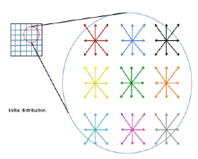
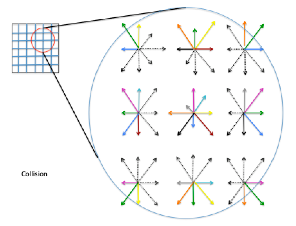
Initializing the package:
In[]:=
CloudImport["https://www.wolframcloud.com/obj/4766c821-ad5b-4a55-9603-9afdf4494e89"]
Setting up the simulation
Setting up the simulation
◼
sAngle represents how close the sail is to the middle line of the boat, with 0 degrees being the sail fully pulled in.
◼
bAngle represents the angle the boat is sailing in relation to the wind, with a lower degree representing a higher angle which points closer to straight up wind.
◼
wind is the velocity of the wind in knots.
In[]:=
sAngle=0;bAngle=45;wind=11;
Reynold's number is used to determine how laminar or turbulent the flow of a liquid is, the higher the number the more turbulent the flow. Reynold's number is calculated by multiplying the wind's velocity by the chord length of the sail (0.001 meters) and dividing by the kinematic viscosity, which I assumed to be 1.5111*10^(-5).
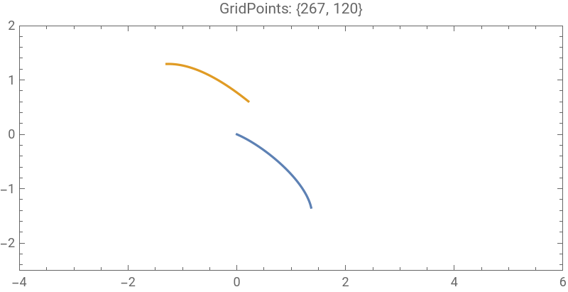
I used trigonometry to position the jib 183 cm in front of the mainsail in the direction of the boat angle.
Initializing the simulation:
In[]:=
state=WindTunnelInitialize[{(wind*0.5144*0.001)/(1.5111*10^(-5)),0.75,0.4},Function[{x,y},{0,0}],{x,-4,6},{y,-2.5,2},t,"CharacteristicLatticePoints"->20,"CharacteristicLatticeVelocity"->wind*0.0008658008658,"TunnelBoundaryConditions"->{"Left"->Function[{x,y,t},{1,0}],"Right"->"Outflow","Top"->"Periodic"},"ObjectsInTunnel"->{ParametricRegion[{0.01{Cos[(-bAngle+sAngle)Degree],-Sin[(-bAngle+sAngle)Degree]},0.01*{Sin[(-bAngle+sAngle)Degree],Cos[(-bAngle+sAngle)Degree]}}.{3((1−t)^2)t*50+3(1−t)(t^2)150+(t^3)*194,3((1−t)^2)t*20+3(1−t)(t^2)*30},{{t,0,1}}],ParametricRegion[{0.01{Cos[(-bAngle+sAngle+10)Degree],-Sin[(-bAngle+sAngle+10)Degree]},0.01*{Sin[(-bAngle+sAngle+10)Degree],Cos[(-bAngle+sAngle+10)Degree]}}.{2(1−jt)jt*50+(jt^2)*163,2(1−jt)jt*37.5+(jt^2)*30}+{-Cos[(bAngle)Degree]*(183*0.01),Sin[(bAngle)Degree]*(183*0.01)},{{jt,0,1}}]}];
I plotted the sails where they would appear in the wind tunnel:
In[]:=
ListLinePlot[state["ObjectsInTunnel"],PlotRange->Evaluate[state["Ranges"]],AspectRatio->Automatic,Axes->False,Frame->True,ImageSize->400,PlotLabel->StringForm["GridPoints: ``",Reverse@state["GridPoints"]],AxesLabel->{"meters","meters"}]
Out[]=
Running the simulation
Running the simulation
In[]:=
ProgressIndicator[Dynamic[state["CurrentTime"]],{0,10}]AbsoluteTiming[WindTunnelIterate[state,10]]
Visualizing the vorticity
Visualizing the vorticity
Vorticity describes the local rotation of a fluid within it's flow. Higher vorticity represents a lower air-pressure and a lower vorticity represents a higher air-pressure.
Calculate the vorticity for each grid point:
Assign colors to different vorticity values:
Darker red colors represent a higher vorticity while darker purple colors represent lower vorticity.
Visualizing the pressure differences
Visualizing the pressure differences
The first graph is the pressure on the jib and the second is the pressure on the main. The lower lines represent the pressure on the windward side (side the wind is directly hitting) and the upper lines represent the pressure on the leeward side (side the wind is past).
jCp represents the pressure coefficient on different points of the jib.
Plot the pressure on the jib:
mCp represents the pressure coefficients on different points of the mainsail.
Plot the pressure on the mainsail:
Lift coefficient is the difference between the pressure above and below a body and is used in the lift formula to determine how effective a body is at generating lift.
In order to calculate the lift coefficient for each sail, I take the difference in the pressure coefficient between the windward and leeward side at the center of effort for each sail (the point where the air pressure is the most concentrated):
After calculating the lift coefficient for each sail, I plug the number into the lift formula to calculate the total lift generated by each sail.
The total surface area of the jib and the main are 3.737945986 and 8.6730190131 respectively.
The density I used is the total number of grid points, (267*120)/(10*4.5)=712.
I added the jib lift and main lift to get the total lift generated.
Calculating the total lift:
Getting my data
Getting my data
Run a simulation for every combination of wind strength, boat angle, and sail angle
Run a simulation for every combination of wind strength, boat angle, and sail angle
Put all the code into one function:
Import the package for all the kernels:
This function took a lot of time to evaluate so I do not recommend running it. I have already provided the data below in the initialization cell:
Cleaning the data
Cleaning the data
Since the sail angle only affects the speed of the boat, I picked the sail angles with the highest lift for each combination of wind strength and boat angle:
In each list, the first element is the wind strength, the second is the sail angle, the third is the boat angle and the last is the total lift generated.
Setting Up the Environment
Setting Up the Environment
Plot the wind vector field to simulate a real life scenario of the wind:
Make a reset function to reset the environment:
Now I can use sailReset[]
Optimizing the Path
Optimizing the Path
Brute force
Brute force
The brute force method is extremely simple yet effective. It requires a high number of iterations of random moves and then picks the best option. In general, brute force can be accurate as long as the number of iterations is high but it is also computationally expensive.
Check all possible moves at each position based on the wind strength:
Function to move the boat in the selected direction and count the time taken to make that move:
Select from the eight possible moves, seven different boat angles and tacking (going in the opposite direction by turning approximately ninety degrees into the direction of the wind):
Randomly choosing a move while preventing the boat from exiting the environment:
Makes the boat randomly move thirty times and counts the final score of the thirty moves (the final distance from the goal plus the total time taken to make those thirty moves plus five times the amount of times it tacks):
This list above shows the path taken. The first item shows the current position and the total time taken to make all the previous moves. The second item shows the angle the boat sailed to get to its current position.
Repeat the above function 100,000 times:
By having a lower score, it means the path taken takes a less amount of time, is closer to the final goal, and makes less tacks.
Choose the path with the lowest score:
Find the total time taken:
Visualize the path taken:
Greedy Algorithm
Greedy Algorithm
The greedy algorithm is another optimization method. It works by evaluating all the possible options in a local area and choosing the option with the lowest score. It is called the greedy method because it often chooses the immediate, short term gains and misses out on the options that require small sacrifices which may lead to long term benefits.
New function that is independent from the previous that does not randomize the tack the boat is on:
Define a way to reset a test position without changing the boat's actual position:
Determine the theoretical distance from goal after making a move:
List the position, time taken, and distance from goal for each possible move:
Choose the move which has the lowest distance from the goal:
Evaluate the best move until the goal is reached:
Clean the list so it can be plotted:
Find the total time taken:
Visualize the path:
Analysis
Analysis
Graph the methods versus time taken:
Plot the two paths side by side:
Looking at the paths the different methods take, it may seem that the greedy algorithm takes a more direct path towards the goal, however it still has a higher time taken compared to the brute force method as each tack has a punishment of 5 seconds. Looking at the wind vector field by itself, I would expect the optimal path to be somewhere on the right as the wind shifts to the right as x increases, therefore lifting the boat angle higher up and decreasing the total distance required to sail. Sailing towards the right side of the course and taking the lift is exactly what the brute force method decided to do.
Graph the boat angle at each move:
Find the mean, median, and mode boat angle:
Looking at the plot and the mean median mode values, the boat tends to oscillate between speed and distance up until the last ten moves where it decides to sail at a lower angle to get to the final destination faster. Oscillating between speed and distance is exactly what happens in a typical race where the general strategy is to go for speed and then use that speed to sail a higher angle for a short period and repeat.
Limitations
Limitations
◼
I did not have exact measurements for my sail dimensions and I eyeballed the sail-shape and angles for both sails. This may result in wind flowing incorrectly past the sails, affecting the final lift calculations. For example, for almost all the combinations of wind-strength and boat-angles, having a sail angle of zero degrees was optimal, which in theory should not be true; a larger sail angle should be more optimal for lower boat angles.
◼
I assumed the sails to be rigid and for current to be nonexistent, which makes the sailboat generate more lift and move faster than theoretically possible.
◼
I used quite a low lattice velocity and very few grid points in my wind tunnel simulations to save on computational time, this may result in less accurate movement of air particles affecting lift calculations.
◼
The wind vector plot is not an accurate representation of wind in real life, with the wind shifts being too controlled and dramatic in angles as well as the wind gradually increasing by a large margin as the boat advanced through the course.
◼
I limited the boat from sailing below x or y equals one which likely caused the boat to sail a slightly less efficient path. In the brute force method, it sailed on starboard for one move before tacking off towards the left although starting on port and sailing straight to the lay-line(imaginary line where you would tack and be able to reach the goal/mark) may have been faster.
Conclusion
Conclusion
Although the simulations and optimization algorithms aren't perfect, this project gave some interesting insights into how my sailboat works and confirmed how different sail headings can affect the lift on the sails. An application I could use for this could be after a day of racing I could import the wind vector data for the day and compare the route I sailed to the optimal route as determined by my algorithms.
Further work
Further work
In the future, there are quite a few improvements I would like to make:
◼
Make the sail measurements fully accurate and implement a third variable called vang which flattens the mainsail.
◼
Introduce downwind by adding the third and largest sail of the boat, the kite.
◼
Introduce a grid search algorithm to find the optimal path.
◼
Use real wind vector data instead of self-made vector fields.
Acknowledgements
Acknowledgements
I want to thank my mentor Daniele for his support as well as teaching assistants Karan, Nicolo, and Sophie.
References
References
Kantor, Ilya. “Bezier Curve.” The Modern JavaScript Tutorial, 30 Nov. 2022, https://javascript.info/bezier-curve.
Mokhasi, Paritosh. “Building a Lattice Boltzmann–Based Wind Tunnel with the Wolfram Language-Wolfram Blog.” Wolfram Blog RSS, 7 Nov. 2019, https://blog.wolfram.com/2019/11/07/building-a-lattice-boltzmann-based-wind-tunnel-with-the-wolfram-language/.
CITE THIS NOTEBOOK
CITE THIS NOTEBOOK
Optimizing paths in sailing through aerodynamics simulations
by Ethan Kong
Wolfram Community, STAFF PICKS, July 13, 2023
https://community.wolfram.com/groups/-/m/t/2963984
by Ethan Kong
Wolfram Community, STAFF PICKS, July 13, 2023
https://community.wolfram.com/groups/-/m/t/2963984