Introduction
Introduction
The devastation wrought by COVID-19 has not spared a single one of the 195 countries in the world. To help contain and fight the virus, each country handled the virus differently, implementing a small or large number of government measures. Some countries, like Japan, only implemented 2 government measures against COVID-19 in 2020. Countries like Hungary, on the other hand, implemented a whopping 67. However, did the number of government measures implemented by each country influence their control of the virus? If so, to what extent did these government measures make a difference? With data about all government measures taken against COVID-19 from each country in 2020, along with statistics about daily new COVID-19 cases and biweekly case growth for each country, we can answer this question.
Getting Government Measures Data
Getting Government Measures Data
We can get data about all government measures implemented in 2020 by country through the Wolfram Data repository.
Import the Coronavirus COVID-19 Pandemic Government Measures dataset:
COVIDData = ResourceData[ResourceObject["Coronavirus COVID-19 Pandemic Government Measures"]]
Out[]=


The dataset gives a variety of information, but what we care about most is in the "Category" column. There are five categories of government measures: public health measures, movement restrictions, social distancing, social and economic measures, and lockdown. Before we get into the details about each type, let's find out how many government measures each country implemented.
Get the amount of government measures implemented by each country by the amount of times the country appears in the dataset:
In[]:=
CountryQuantity = Sort[Counts[Normal[COVIDData[All,"Country"]]]];
Example outputs:
Out[]=
34,35,35,35,35,38,39,51,55,67
Visualize these quantities on a bar chart:
BarChart[CountryQuantity,PlotTheme->"Business",PlotLabel->"Amount of Government Measures Implemented by Countries in 2020"]
Out[]=
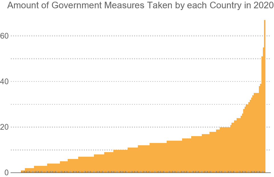
As shown by the bar chart, there is a pretty wide distribution in quantity of government measures implemented in each country. The majority took 0-20, with other some countries taking 20-70. Now that we know the general quantity of measures implemented, we can find what types of measures countries implemented the most and the least.
Get the total amount of measures implemented by all countries:
In[]:=
CategoryQuantity = Reverse[Sort[Counts[DeleteMissing[Normal[COVIDData[All,"Category"]]]]]];
Create a function to visualize the proportion of category quantities on a pie chart:
In[]:=
PChart[data_,countries_]:=PieChart[N[data/Total[data]],ChartStyle->"Pastel",LabelingFunction(Placed[Row[{NumberForm[100#,{3,1}],"%"}],"RadialCallout"]&),ChartLegendsAutomatic,ImageSize->Medium,PlotLabel->"Percentage of Government Measures Taken by "<> countries <> " in 2020"]
Visualize these proportions:
In[]:=
PChart[CategoryQuantity,"All Countries"]
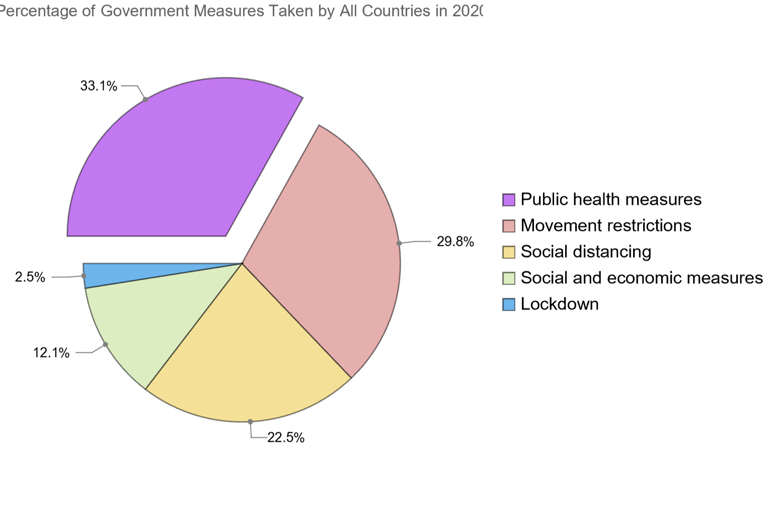
The types of government measures implemented by countries is spread out as well. For the most part, countries implemented public health measures, movement restrictions, and social distancing, but some implemented social and economic measures and lockdowns. It's interesting to see what categories the world focused their efforts against COVID-19 on, and we will be able to see the extent of these efforts.
Visualizing Government Measures on a World Map
Visualizing Government Measures on a World Map
Although we get crucial information from the bar chart, we don't know which countries implemented how many government measures. Visualizing these quantities on a world map would be far more detailed and easier to analyze, so let's do that.
Visualize worldwide government measures distribution on a world map:
GeoRegionValuePlot[CountryQuantity,PlotLabel"Amount of Total Government Measures per Country",ImageSizeLarge]
Out[]=
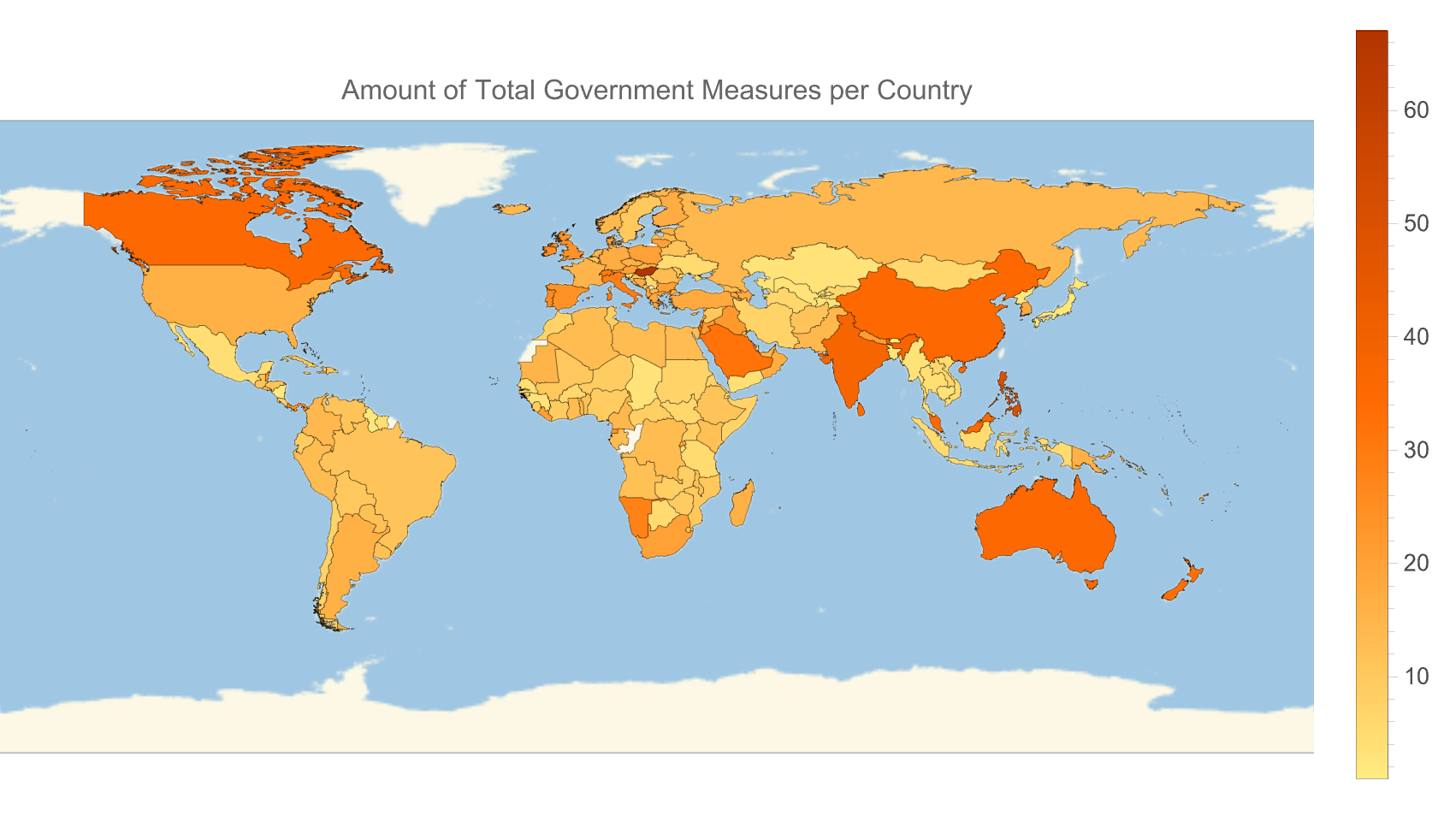
With the GeoRegionValuePlot, we can easily identify which countries took a lot of measures, and which took fairly little. We can take this plot a step further, though, by visualizing the quantities of measures implemented for the specific categories: Public health measures, social and economic measures, movement restrictions, social distancing, and lockdown. Doing this is rather simple because we can filter the dataset to get only measures of a certain category.
Find the amount of government measures taken by each country from only a specific category:
In[]:=
GetCategoryCountries[category_]:=Counts[Normal[COVIDData[Select[#Category==category&],{"Country"}][All,"Country"]]]
Applying this function to the 5 different category types will give us the necessary quantities.
Example output of the quantity of public health measures taken from 10 countries:
Let's visualize all of these quantities on a geo map now.
We get a lot of information from these plots. China seems to have implemented a large number of public health measures. Saudi Arabia ordered an unusually high amount of movement restrictions. Italy implemented an unparalleled number of lockdowns. We'll see if these had any impact on how well they handled the virus.
Visualizing Government Measures with Respect to Time
Visualizing Government Measures with Respect to Time
The quantity and proportion of government measures implemented by each country are important to know, however, it is vital to know when these measures were implemented. Fortunately, the dataset gives us an implementation date for each government measure.
Since there are too many measures to visualize on a single timeline, it is smarter to get 5 different timelines for each of the 5 types of measures implemented, and compare them to each other.
Get all the implementation dates of any specific government measure:
Applying this function to the 5 different category types will give us the desired information.
Example output of 10 implementation dates for country lockdowns:
Now that we have all the implementation dates, sorted by type of government measure, we can visualize them on a timeline.
Visualize implementation dates on a timeline plot:
It's interesting that most countries took public health measures, social and economic measures, and movement restrictions starting in January, but for the most part, didn't implement social distancing or lockdowns until March. We'll see if the timing of implementation of these government measures had any effect on a countries handling of COVID-19, and to what extent.
Getting COVID-19 Daily Percent Growth Data
Getting COVID-19 Daily Percent Growth Data
All we needed from the government measures dataset were measures implemented and implementation dates. Now that we've gotten that data, we can look at the daily COVID-19 cases dataset. The dataset is from "Our World In Data", and will be linked at the bottom.
Import the daily cases COVID-19 dataset:
Since we only care about the daily new cases and the date they were reported, those are what we will extract from the dataset.
Filter dataset to only get data about a specific country (Afghanistan is used as an example):
Extract the dates of all new cases reports in Afghanistan.
Example outputs:
Extract the new cases reports in Afghanistan:
Right now, the newcases variables is storing the raw number of new cases reported each day. It wouldn't make much sense to visualize these numbers now, since there are countless sources online that have already done this, and it wouldn't tell us much anyway. A better indicator of a countries handling of the virus, along with when they had outbreaks, would be to get the percent growth in daily new cases.
Get the percent change of a list of numbers and apply it to to newcases:
Finally, we can transpose the dates and daily percent change in cases, and put this matrix into a time series to visualize later.
Transpose dates and new cases and put in a time series:
To make this process more efficient, we can generalize all these steps into a single function:
Get the daily percent growth time series for any country:
Visualizing Daily Percent Growth Data
Visualizing Daily Percent Growth Data
If we visualized the daily percent growth right now, here's what the plot would look like:
This plot just seems like a pencil scribble, and we don't even know the implementation dates or types of government measures implemented in Afghanistan, which are critical to this plot. Let's do that now.
Create a visual label for each government measure, color-coded, timestamped, and visualized nicely:
This function creates a graphic data point for measures implemented which we will pass into an epilog. Let's get the country plot now.
Get the daily percent growth of a country, with government measure implementation dates shown:
With the government measures labeled on the graph, along with necessary details indicated, we can visualize the daily percent growth plot for any country. As examples, here are the plots of the country we used previously, Afghanistan, and Italy.
It's clear Afghanistan implemented less government measures than Italy, and as a result, their percent growth in new COVID-19 cases is far more volatile. Italy's government measures, along with the many lockdowns they ordered, seem to have done a great job controlling the spread of the virus throughout the year, with only a few slip-ups inJune.
Getting Biweekly Percent Growth and Visualizing it
Getting Biweekly Percent Growth and Visualizing it
The daily percent growth of COVID-19 cases in any country can tell us a lot about how well they can manage COVID-19 outbreaks, given their government measures. However, we shouldn't interpret it as the ultimate deciding factor for how well a country handled the virus. Getting biweekly percent growth of COVID-19 cases is an additional insight to a countries handling of the virus, and may also be a more reliable way to measure handling than daily percent growth.
It wouldn't be hard to just convert the daily cases dataset into biweekly percent growth, however the "Our World In Data" organization already has a dataset of biweekly case growth, so we will use that. This dataset will be linked at the bottom as well.
Import the biweekly case growth dataset:
What's great is that this dataset already converted the raw numbers to percent change, maintaining the same dataset format, so we can recycle our code and plot it efficiently.
Get the time series of a countries biweekly percent growth:
Get the biweekly percent growth plot of a country:
Just like that, we're done. Here are the biweekly case growth plots for the countries we used previously, Afghanistan and Italy.
For both countries, biweekly case growth percentages were through the roof for the first few months of 2020. They mostly stayed on the plot for the rest of the year, however it's interesting that Italy now has more volatile plot. It's likely they implemented so many measures because the COVID-19 situation was severe in early 2020, and this plot highlights that.
Putting it all Together
Putting it all Together
It's hard to look at all the information we just gathered individually, so we should organize the information into a single function call. Doing so will also make it much easier to analyze outbreak and government measures statistics about a certain country.
Before coding, though, we need to decide what qualifies as an 'outbreak'. There are many different ways of evaluating the definition of an outbreak, but a simple and fair way would be if a countries daily or biweekly growth at one point in time is more than double the previous data point, meaning growth is at least 100%. We can easily find the number of weekly and daily outbreaks any country had in 2020 with this categorization.
Get the number of biweekly outbreaks in a country in 2020
Get the number of daily outbreaks in a country in 2020:
It's also necessary to find the total amount of government measures implemented in a country.
Get the number of government measures implemented in a country in 2020:
Now that we have all the necessary functions created, let's organize the information.
Organize all relevant info about a countries outbreak and COVID-19 cases statistics:
Just like that, we're done. Here's an example output of the outbreak and government measures statistics of China:
If we want to find get this data for any country without using code, we can create and input form. Try it out.
Classifying Countries by their Number of Outbreaks and COVID-19 Case Growth
Classifying Countries by their Number of Outbreaks and COVID-19 Case Growth
With all this information collected, we can now try to find the correlation between a countries number of daily/biweekly outbreaks to the number of government measures it implemented. Of course there is a correlation between daily and biweekly outbreaks, so the main point of focus with this sectoin is the relationship between government measures and outbreaks. It's obvious government measures aren't the only factor that determine outbreaks in a country, but they play a big enough role to offer key insight.
Using machine learning with inputs of the number of daily outbreaks, biweekly outbreaks, and government measures implemented in a country, we can find clusters in the data, and visualize these clusters with a feature space plot.
Create an association of country biweekly outbreaks, daily outbreaks, and government measures as input data to output continent color:
Example outputs of 3 countries on different continents:
These example outputs highlight a problem we might run into when visualizing on a feature space plot. Since the feature space plot uses the values of an association as visual labels, it would be overwhelming to display the text of 195 countries. Visualizing the countries by a single single-colored data point also wouldn't work, since we might find clusters in the data, but we would have no idea which country was which. An easy way we can visualize the data points with sufficient information is to color-code the countries by continent.
Get all countries in a specific continent:
Get all countries in the dataset:
Color code a country by what continent it is located in:
With the color-coding function set up, we can improve our previous function to output a certain color label as an association value.
Example output of the previous 3 countries:
With out association finalized, we can get the country stats, sorted by continent, for all countries, and plot them on a feature space plot.
Get the country stats, sorted by continent, for all countries:
Plot the country stats on a feature space plot:
Although this plot may seem like a burst of confetti at first, it actually gives us important information. The most notable part of this plot is the divided section of points to the top right. Countries of all continents are here, and it is likely those are the countries that had little daily or biweekly outbreaks and similar number of government measures implemented. Furthermore, there is a very tight cluster of green points, indicating that countries in Oceania had very similar outbreak and/or government measure statistics. In the main plot to the bottom left, there also appears to be a faint correlation between yellow and blue data points, or countries in Asia and Europe. There is no definitive cluster, however many smaller clusters appear throughout the plot consisting of these colored points. On the other hand, there is no glaring patterns or clusters with countries in Africa, North America, and South America. It's interesting why this might be the case.
Perhaps there are other ways of color-coding the data that may provide us more insight on the correlation between the number of outbreaks in a country and the amount of government measures it implemented, like the outbreaks or government measures themselves. For example, the more outbreaks or government measures in a country, the colder the associated color.
But how can we assign a color based on a number? First, we need to scale the outbreak or government measure quantities to a range of 0 to 1 for all countries, then assign the hue function to that value. Doing so will give us a gradient scale from red, all the way to purple, then pink, and back to red.
Visualizing with Government Measures Color-coding
Visualizing with Government Measures Color-coding
Color-code a country based on the number of government measures it implemented, warm colors being less, cold colors being more:
Create an association of country biweekly outbreaks, daily outbreaks, and government measures as input data to output government measures color:
Example outputs of Bolivia and Germany:
Get the country stats, sorted by quantity of government measures, for all countries:
Plot the country stats on a feature space plot:
This feature plot certainly shows more patterns in the data. On the top right, there are several countries which took 0 measures and all have similar outbreak statistics, as shown by how closely grouped they are. However, not all countries that took 0 government measures fit the pattern. There are many red dots scattered on the outside of the main plot. It also appears that the points are color-coded to form a sort of spiral rainbow, with red on the outside, and blue/purple at the center. There is no strong correlation between points of the same color, however it is clear they are grouped with each other more so than with points of a different color. This does give insight that countries that took a certain number of government measures also had similar number of biweekly and daily outbreaks. Let's check out if the outbreak quantities have any correlation now.
Visualizing with Biweekly Outbreaks Color-coding
Visualizing with Biweekly Outbreaks Color-coding
Color-code a country based on the number of biweekly outbreaks it had, warm colors being less, cold colors being more:
Create an association of country biweekly outbreaks, daily outbreaks, and government measures as input data to output biweekly outbreaks color:
Example outputs of Sudan and Papua New Guinea:
Get the country stats, sorted by quantity of biweekly outbreaks, for all countries:
Plot the country stats on a feature space plot:
By color-coding the data points by quantity of biweekly outbreaks, we see a very strong rainbow gradient pattern on the feature space plot. Countries that had 0 biweekly outbreaks are almost entirely clustered together on the top right, showing a very strong correlation between the number of biweekly outbreaks to number of daily outbreaks and government measures in a country. Looking at the majority part of the plot, the data points are still quite spread out, however they are almost all entirely surrounded by other points of similar colors. This plot lets a deduce that the number of biweekly outbreaks in a country is a strong indication of the number of government measures implemented and daily outbreaks in a country. Let's see if there is such a strong pattern with daily outbreak color-coding.
Visualizing with Daily Outbreaks Color-coding
Visualizing with Daily Outbreaks Color-coding
Color-code a country based on the number of daily outbreaks it had:
Create an association of country biweekly outbreaks, daily outbreaks, and government measures as input data to output daily outbreaks color:
Example outputs of Jamaica and India:
Get the country stats, sorted by quantity of daily outbreaks, for all countries:
Plot the country stats on a feature space plot:
Just like in the biweekly color-coded plot, there is a rainbow gradient pattern on the daily outbreaks plot. We see the same red cluster to the top right, telling us once again that a low number of daily outbreaks indicates similar number of biweekly outbreaks and government measures implemented for countries, however, there is slight difference in the rainbow gradient pattern in this plot. In the biweekly outbreak plot, the gradient pattern ran right to left, whereas in this plot, the gradient runs top to down. The data points also appear to be more clustered at the bottom, where countries that had a high number of daily outbreaks are located. This feature space plot perhaps tells us the most information of all: there is indeed a correlation between the number of daily outbreaks to the number of biweekly outbreaks and government measures implemented in a country, and this correlation strengthens with more daily outbreaks.
Conclusion
Conclusion
Using a variety of datasets from the Wolfram data repository and online, we found patterns in the number of biweekly outbreaks, daily outbreaks, and government measures implemented for each country. We found that the more biweekly or daily outbreaks in countries, the more closely their quantity of government measures and other information resembled one another. However, the quantity of government measures implemented does not necessarily indicate the number of biweekly or daily outbreaks in a country. Furthermore, there was little correlation between a country’s outbreak, government measures statistics, and which continent it was located in, except Oceania. This lack of correlation indicates that location did not strongly influence how countries handled the virus. Finding a correlation between outbreaks and government measures wasn’t the only thing we did, in any case. Now that we are almost at the start of the Fall of 2021(at the time of writing this), it is clear which countries did a better job controlling the virus than others. Likely, the daily and biweekly outbreak plots we graphed for countries in 2020 foreshadowed their COVID-19 situation for 2021. Therefore, it is likely that the type of government measures implemented in each country influenced its COVID-19 situation for 2021. Hopefully, this project gave a new and detailed approach to analyzing the COVID-19 situation and governments’ role in controlling the virus in their country.
Extensions
Extensions
Even though it would be quite complicated, it would be fascinating to find correlation in the number of outbreaks in a country to the type of government measure implemented. Did countries that implemented a larger number of public health measures have a similar number of outbreaks? Or did countries that implemented lockdowns have a similar number of outbreaks?
It would also be interesting to do this project, but for 2021 COVID-19 statistics, and compare them to the 2020 ones. Unfortunately, there is only data available about government measures for 2020, so that is what was analyzed in this project. Should data come out for 2021, though, this idea would be easily implementable and even more insightful.
It would also be interesting to do this project, but for 2021 COVID-19 statistics, and compare them to the 2020 ones. Unfortunately, there is only data available about government measures for 2020, so that is what was analyzed in this project. Should data come out for 2021, though, this idea would be easily implementable and even more insightful.