A total of 100 randomly distributed feed compositions were generated within the ternary composition space of methanol–heptane–hexane and analyzed using the Tangent Plane Distance (TPD) criterion coupled with the NRTL activity coefficient model. For each feed composition z, the global minimum value of the TPD function was determined through numerical optimization.
The TPD criterion provides a rigorous thermodynamic test for phase stability. A negative minimum TPD value (TPDmin < 0) indicates that the Gibbs free energy surface can be lowered by forming an additional liquid phase, implying that the feed composition is thermodynamically unstable and a liquid–liquid phase split is expected. Conversely, a positive minimum TPD value (TPDmin > 0) signifies that the mixture is stable and remains as a single liquid phase.
In the ternary diagram, red points represent feed compositions for which TPDmin < 0, corresponding to the two-phase liquid–liquid equilibrium region, while cyan points denote compositions with TPDmin > 0, corresponding to the single-phase region. To avoid misclassification caused by numerical round-off errors during optimization, a small tolerance threshold (here we take -0.001) was applied. This threshold distinguishes genuinely negative TPD values from numerical noise near zero, ensuring reliable identification of stable and unstable compositions.
The resulting distribution of stable and unstable points clearly outlines the phase behavior predicted by the NRTL model and provides a numerical validation of the liquid–liquid equilibrium region within the ternary system.
LLE diagram using the method based on common tangent plane and arc-length continuation
ClearAll["Global`*"];
Universal gas constant
R=1.9872041;
Temperature
T=273.15+32.85;
NRTL PARAMETERS
a13=0.42399900;a12=0.301800;a32=0.440800;t31=1287.78000;t13=1915.07700;t23=1598.3120000;t32=1566.43700;t12=-285.9411;t21=252.997600;α={{0.,a12,a13},{a12,0.,a32},{a13,a32,0.}};τ={{0.,t12,t13},{t21,0.,t23},{t31,t32,0.}}/(RT);
In[]:=
α//MatrixForm
Out[]//MatrixForm=
0. | 0.3018 | 0.423999 |
0.3018 | 0. | 0.4408 |
0.423999 | 0.4408 | 0. |
In[]:=
τ//MatrixForm
Out[]//MatrixForm=
0. | -0.470233 | 3.14936 |
0.416057 | 0. | 2.62844 |
2.11777 | 2.57602 | 0. |
G[i_,j_]:=Exp[-α[[i,j]]τ[[i,j]]];
COMPOSITION VECTOR
xvec[x1_,x2_]:={x1,x2,1-x1-x2};
NRTL ACTIVITY COEFFICIENTS
lnGamma[i_,x1_,x2_]:=Module[{x,term1,term2},x=xvec[x1,x2];term1=Sum[x[[j]]τ[[j,i]]G[j,i],{j,1,3}]/Sum[x[[k]]G[k,i],{k,1,3}];term2=Sum[x[[j]]G[i,j]/Sum[x[[k]]G[k,j],{k,1,3}](τ[[i,j]]-Sum[x[[m]]τ[[m,j]]G[m,j],{m,1,3}]/Sum[x[[m]]G[m,j],{m,1,3}]),{j,1,3}];term1+term2];gamma[i_,x1_,x2_]:=Exp[lnGamma[i,x1,x2]];
DIMENSIONLESS GIBBS ENERGY OF MIXING: g/RT
gmix[x1_,x2_]:=Module[{x},x=xvec[x1,x2];Sum[x[[i]]Log[x[[i]]],{i,1,3}]+Sum[x[[i]]lnGamma[i,x1,x2],{i,1,3}]];
DERIVATIVES
dgdx1[x1_,x2_]:=Evaluate[D[gmix[u,v],u]/.{u->x1,v->x2}];dgdx2[x1_,x2_]:=Evaluate[D[gmix[u,v],v]/.{u->x1,v->x2}];
UNKNOWNS
vars={x1a,x2a,x1b,x2b,m1,m2};
COMMON TANGENT EQUATIONS
eq1=dgdx1[x1a,x2a]==m1;eq2=dgdx1[x1b,x2b]==m1;eq3=dgdx2[x1a,x2a]==m2;eq4=dgdx2[x1b,x2b]==m2;eq5=gmix[x1b,x2b]-gmix[x1a,x2a]==m1(x1b-x1a)+m2(x2b-x2a);
EXTRA CONSTRAINT - Prevent trivial solution xα=xβ
eq6=(x1b-x1a)^2+(x2b-x2a)^2==d;
first value for d --- very small d=0.001 yield approximately the plait point
d0t=0.07;
solution
solct=FindRoot[{eq1,eq2,eq3,eq4,eq5,eq6/.d->d0t},{{x1a,0.33},{x2a,0.4},{x1b,0.060},{x2b,0.4},{m1,-0.65},{m2,-0.45}},MaxIterations->1000]
Out[]=
{x1a0.0100149,x2a0.882978,x1b0.00706729,x2b0.618419,m1-4.54248,m20.0315688}
In[]:=
init={x1a[0]==(x1a/.solct),x2a[0]==(x2a/.solct),x1b[0]==(x1b/.solct),x2b[0]==(x2b/.solct),m1[0]==(m1/.solct),m2[0]==(m2/.solct),d[0]==d0t}
Out[]=
{x1a[0]0.0100149,x2a[0]0.882978,x1b[0]0.00706729,x2b[0]0.618419,m1[0]-4.54248,m2[0]0.0315688,d[0]0.07}
In[]:=
initdev={x1a'[0]==0.01,x2a'[0]==0.01,x1b'[0]==0.01,x2b'[0]==0.01,m1'[0]==0.01,m2'[0]==0.01,d'[0]==0.01}
Out[]=
{[0]0.01,[0]0.01,[0]0.01,[0]0.01,[0]0.01,[0]0.01,[0]0.01}
′
x1a
′
x2a
′
x1b
′
x2b
′
m1
′
m2
′
d
In[]:=
SYS={eq1,eq2,eq3,eq4,eq5,eq6}/.x1a->x1a[s]/.x1b->x1b[s]/.x2a->x2a[s]/.x2b->x2b[s]/.m1->m1[s]/.m2->m2[s]/.d->d[s];
In[]:=
Length@init
Out[]=
7
In[]:=
Length@initdev
Out[]=
7
In[]:=
Length[SYS]
Out[]=
6
In[]:=
auxeq=x1a'[s]^2+x1b'[s]^2+x2a'[s]^2+x2b'[s]^2+m1'[s]^2+m2'[s]^2+d'[s]^2==1
Out[]=
2
′
d
2
′
m1
2
′
m2
2
′
x1a
2
′
x1b
2
′
x2a
2
′
x2b
In[]:=
SYSFinal=Join[SYS,{auxeq},init,initdev];
In[]:=
Length@SYSFinal
Out[]=
21
In[]:=
SOL=NDSolve[SYSFinal,{x1a,x2a,x1b,x2b,m1,m2,d},{s,-100,100},AccuracyGoal->5]
Out[]=
x1aInterpolatingFunction,x2aInterpolatingFunction,x1bInterpolatingFunction,x2bInterpolatingFunction,m1InterpolatingFunction,m2InterpolatingFunction,dInterpolatingFunction


In[]:=
DATA1=Table[{x1a[s],x2a[s],1-x1a[s]-x2a[s]}/.SOL,{s,-7.84,16.05,0.01}];DATA2=Table[{x1b[s],x2b[s],1-x1b[s]-x2b[s]}/.SOL,{s,-7.84,16.05,0.01}];
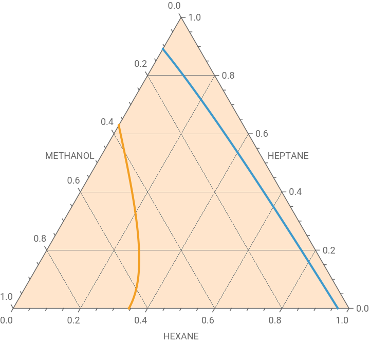
Type II liquid-liquid equilibrium (LLE) diagram
In[]:=
p0=Show[TernaryListPlot[{Flatten[DATA1,1],Flatten[DATA2,1]},Joined->True,PlotStyle->Thick,GridLines->Automatic,FrameLabel->{"HEXANE","HEPTANE","METHANOL"},PlotRange->All,Method->{"Backdrop"->LightOrange}]]
Out[]=
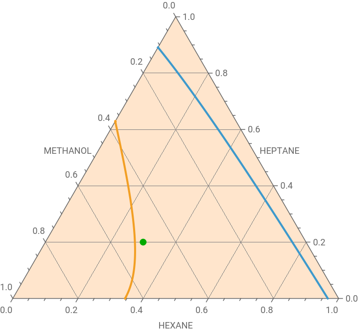
TANGENT PLANE DISTANCE (TPD) ANALYSIS - case 1 : Liquid-liquid phase split expected
TANGENT PLANE DISTANCE (TPD) ANALYSIS - case 1 : Liquid-liquid phase split expected
TANGENT PLANE DISTANCE (TPD) ANALYSIS FOR TERNARY LLE
FEED COMPOSITION
z={0.30,0.20,0.50};
In[]:=
Pt={{2,1},{0,Sqrt[3.]}}/2;
In[]:=
Show[p0,Graphics[{Darker@Green,PointSize[0.02],Point[Pt.{z[[1]],z[[2]]}]}]]
Out[]=
NRTL ACTIVITY COEFFICIENTS
FEED ACTIVITY COEFFICIENTS
TPD FUNCTION
GLOBAL MINIMUM OF TPD
RESULTS
TANGENT PLANE DISTANCE (TPD) ANALYSIS - case 2 : Single liquid phase
TANGENT PLANE DISTANCE (TPD) ANALYSIS - case 2 : Single liquid phase
TANGENT PLANE DISTANCE (TPD) ANALYSIS FOR TERNARY LLE
FEED COMPOSITION
FEED ACTIVITY COEFFICIENTS
TPD FUNCTION
GLOBAL MINIMUM OF TPD
RESULTS
TANGENT PLANE DISTANCE (TPD) ANALYSIS - case 3 : 100 randomly selected feed compositions
TANGENT PLANE DISTANCE (TPD) ANALYSIS - case 3 : 100 randomly selected feed compositions
TANGENT PLANE DISTANCE (TPD) ANALYSIS yields expected results with cyan dots (single-phase region and positive TPD minimum) and red dots (two-phase region and negative TPD minimum)
CITE THIS NOTEBOOK
CITE THIS NOTEBOOK
TPD stability analysis of random feed compositions
by Housam Binous and Ahmed Bellagi
Wolfram Community, STAFF PICKS, June 9, 2026
https://community.wolfram.com/groups/-/m/t/3729753
by Housam Binous and Ahmed Bellagi
Wolfram Community, STAFF PICKS, June 9, 2026
https://community.wolfram.com/groups/-/m/t/3729753