We study the one-dimensional heat conduction equation on the half-line, subject to Dirichlet boundary conditions:
u
t
u
xx
(
1
)u(x,0),0<x<∞
-x
e
(
2
)u(0,t)cos(t),t>0
(
3
)We compute the Fourier transform of (x) on the half-line
u
0
-x
e
u
1
1+iλ
and (t)cos(t)
g
0
g
0
1
2
(λ+i)t
e
λ+i
(λ-i)t
e
λ-i
The contour can be any curve between the real axis and the .
+
C
∂
+
D
We choose the following trapezoidal contour
+
C
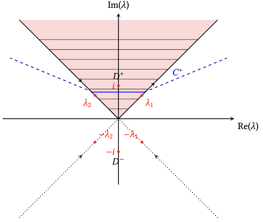
Thus, the solution reduces to:
u(x,t)++iλ+i+-iλ.
1
2π
∫
+
C
iλx-t
2
λ
e
1
1+iλ
1
iλ-1
1
2
λ
1
2
λ
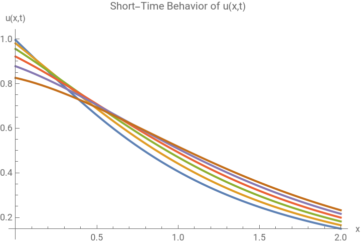
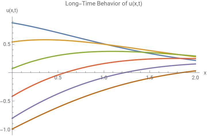
To better understand the temporal evolution of the solution , we numerically evaluated and plotted the function for various values of using the trapezoidal contour implementation.
u(x,t)
t
Define the complex-valued function V(k,x,t)
v[k_,x_,t_]:=-I*1/2*Exp[I*k*x-k^2*t]*(1/(k-I)+1/(k+I)-k*(1/(k^2+I)+1/(k^2-I)))/Pi
Set L value
l=3/4;
Define the three contours k1,k2,k3
k1[r_]:=l+(3/4)*I+r*Exp[I*Pi/6];k2[r_]:=-l+(3/4)*I+r*Exp[I*5*Pi/6];k3[s_]:=s+(3/4)*I;
Derivatives of the contours
dk1[r_]:=D[k1[r],r];dk2[r_]:=D[k2[r],r];dk3[s_]:=D[k3[s],s];
Define the approxU function with NumericQ guards
approxU[x_?NumericQ,t_?NumericQ]:=Module[{temp1,temp2},temp1=NIntegrate[Re[v[k1[r],x,t]*dk1[r]-v[k2[r],x,t]*dk2[r]],{r,0,Infinity},AccuracyGoal->6,PrecisionGoal->6,MaxRecursion->20];temp2=NIntegrate[Re[v[k3[s],x,t]*dk3[s]],{s,-l,l},AccuracyGoal->6,PrecisionGoal->6,MaxRecursion->20];temp1+temp2]
Example: Evaluate at a point
approxU[0.5,0.1]
Out[]=
0.658113
Step 4: Plot the 3D surface
Plot3D[approxU[x,t],{x,0,3},{t,0,2Pi},AxesLabel->{"x","t","u(x,t)"},PlotLabel->"Fokas Method Solution of Half-Line Heat Equation",Mesh->None]
Out[]=

In[]:=
Table[approxU[0,t],{t,0,0.6,0.1}]
Out[]=
{1.,0.995004,0.980067,0.955336,0.921061,0.877583,0.825336}
With[{times={0.1,0.2,0.3,0.4,0.5,0.6},styles=ColorData[97,"ColorList"]},Plot[Evaluate[Join[Table[approxU[x,t],{t,times}],{u[x,0]}]],{x,0,2},PlotStyle->Join[styles[[;;Length[times]]],{{Black,Dashed}}],PlotLegends->LineLegend[Join[Table["t = "<>ToString[t],{t,times}],{"t = 0"}],LegendLabel->"Short-Time Behavior"],AxesLabel->{"x","u(x,t)"},PlotLabel->"Short-Time Behavior of u(x,t)"]]
Out[]=


In[]:=
With[{times={0.5,1,1.5,2,2.5,3},styles=ColorData[97,"ColorList"]},Plot[Evaluate[Join[Table[approxU[x,t],{t,times}],{u[x,0]}(*Thisisu(x,0)*)]],{x,0,2},PlotStyle->Join[styles[[;;Length[times]]],(*applydistinctcolorpert*){{Black,Dashed}}(*styleforu(x,0)*)],PlotLegends->LineLegend[Join[Table["t = "<>ToString[t],{t,times}],{"u(x,0)"}],LegendLabel->"Long-Time Behavior"],AxesLabel->{"x","u(x,t)"},PlotLabel->"Long-Time Behavior of u(x,t)"]]
Out[]=
CITE THIS NOTEBOOK
CITE THIS NOTEBOOK
Application of the unified transform (Fokas method) to the one-dimensional heat equation on the half line
by Athanasios Paraskevopoulos
Wolfram Community, STAFF PICKS, December 23, 2025
https://community.wolfram.com/groups/-/m/t/3595944
by Athanasios Paraskevopoulos
Wolfram Community, STAFF PICKS, December 23, 2025
https://community.wolfram.com/groups/-/m/t/3595944