ABSTRACT: A new method for phase recovery from a single two-beam interferogram is presented. Conventional approaches, relying on trigonometric inversion followed by phase unfolding and unwrapping, are hindered by discontinuities typically addressed through intricate algorithms. Our method bypasses the traditional unfolding and unwrapping, instead formulating a first-order differential equation directly relating the phase to the interferogram. Integration of this equation enables continuous retrieval of phase along the straight path. This approach accommodates both the Newton- and Fizeau-type interferograms. CITATION (original article): V. Berejnov, B. Y. Rubinstein (2025), Continuous Recovery of Phase from Single Interferogram, arXiv:2509.06299. https://doi.org/10.48550/arXiv.2509.06299
Introduction
Introduction
When a reference beam and an object beam—both monochromatic and coherent—overlap in space, they interfere with each other. Placing a detector, photographic film, or photographic plate in this region allows the interference pattern to be recorded as a series of monochromatic fringes, ranging from dark to bright. This recorded pattern, known as an interferogram, encodes the spatial variation of the phase difference between the two interfering beams.
In practical applications, this phase difference can be converted into an optical path difference, which relates either to: (i) the surface shape z(x,y) of the object, if the object beam is reflected, or (ii) the material density variation ρ(x,y) of the object, if the object beam passes through it. In both cases, retrieving the phase difference from the interferogram is a crucial step.
We propose a direct differential method to decode the interferogram and retrieve the phase along any straight path [1]. For simplicity, we consider the interference of two parallel monochromatic beams, where the interferogram gray function G, representing the recorded fringe intensity, is given by
G(x,y) = A(x,y) + B(x,y) cos φ(x,y). (1)
To isolate the phase contribution, it is convenient to introduce the normalized interferogram function F
F(x,y) = [G(x,y) - A(x,y)] / B(x,Y), (2)
which depends only on the phase:
F(x,y) = cos φ(x,y). (3)
To retrieve the phase from F, rather than performing the traditional inversion in Eq. (3), we differentiate Eq. (3); squaring both the result and Eq. (3), summing them up, and eliminating the trigonometric functions by applying the Pythagorean identity, we obtain the differential equation:
2
φ'x,
y
2
F'x,
y
2
Fx,
y
where the derivative is taken along the x-axis while y is held constant, denoted by (Eq.(4) holds also when the derivative is taken along y-axis while x is held constant). This differential equation (4) permits, in general, direct retrieval of the phase from the given interferogram by using Eq.(2) as an input. Introducing K
y
K(x,) =/ , (5)
y
F'x,
y
1-
2
Fx,
y
we write the differential equation (4) for the phase retrieval as
φ’(x,) = K(x,) . (6)
y
y
Solving Eq. (6) involves integration of K along a series of x-segments, each corresponding to a region where the phase derivative has a constant sign. Since the sign of the phase derivative follows a simple alternating sequence, {1,−1,1,−1,…} or its inverse,
{−1,1,−1,1,…}, the integration proceeds without difficulty, provided the x-segment boundaries where the phase derivative changes sign are properly identified. They are determined by the roots corresponding to the extrema of the equation
{−1,1,−1,1,…}, the integration proceeds without difficulty, provided the x-segment boundaries where the phase derivative changes sign are properly identified. They are determined by the roots corresponding to the extrema of the equation
2
Kx,
y
which must be found either analytically or numerically. From all roots, the extrema {} must be identified, which, together with the boundaries of the interferogram, define the integration intervals. In this framework, the phase retrieval process reduces to sequentially obtaining the phase for the i-th segment according to the following formula:
χ
i
φ
i
y
Φ
i-1,
y
σ
x,i
x
∫
χ
i
here, the term denotes the phase value at the (i−1)-th segment, while takes the value 1 or −1 according to the chosen sign sequence. The phase at the left end of the first x-segment is defined by the boundary phase φ(0,) (0 here corresponds to the edge of the interferogram: ), which can be determined using the equation similar to Eq. (4). In the case of φ(0,) the term ,i-1 at the edge of the first y-segment reduces to the single value φ(0,)≡φ(,), which can be obtained directly from the interferogram using Eq. (3).
Φ
i-1,
y
σ
x,i
y
x=
x
min
y
Φ
x
0
x
min
y
min
Details of this mathematical framework, along with analytical and numerical examples, are presented in [1].
Here, we demonstrate the process of phase recovery. We begin by creating the interferogram G(x,y)=1 + cos ϕ(x,y), where ϕ(x,y) is a given “seed” phase describing the interferogram of two parallel, flat interfering beams simplified by assuming A=B=1, corresponding to homogeneous background illumination and a noise-free case. From the G(x,y) array, which mimics the image, we construct the corresponding interferogram function F(x,y). By taking several slices of F along the x-axis and interpolating F into a continuous functional form, we solve the differential equation described above and retrieve the series of phase profiles combined into the phase φ(x, ) for each F-slice.
y
In [1], a variety of synthetic interferogram examples were considered, including:
Parabolic phase: single extremum root along x and y;
Hyperbolic phase: single extremum root along x and y;
Hyperbolic phase with inflection: single extremum root along x and inflection along y;
Warped type 1: two extremum roots along x and one extremum root along y, no inflection;
Warped type 2: two extremum roots along x with a flat inflection, and one extremum root along y;
Gaussian phase: single extremum root along x and y;
Gaussian with linearly modulated phase: no roots.
In this presentation, we compute phases of three distinctly different interferograms from [1].
Reference
[1] V. Berejnov and B. Y. Rubinstein, Continuous Recovery of Phase from Single Interferogram, 2025, https://arxiv.org/abs/2509.06299
Input: Phase and its visualization
Input: Phase and its visualization
1. Seed phases ϕ
1. Seed phases ϕ
Three types of the seed phases, which can be evaluated independently using the code presented.
1.1 ϕ(x,y)=1+A13x-2(B1+A2x)+B22y
1.1
ϕ(x,y)=1+
A
1
3
x
-+
2
(+x)
B
1
A
2
B
2
2
y
1.2 ϕ(x,y)=2x-2y
1.2
ϕ(x,y)=-
2
x
2
y
1.3 ϕ(x,y)=A1-B12x+2y+B2(x+R)
1.3
ϕ(x,y)=+B2(x+R)
A
1
-+
B
1
2
x
2
y
2. Selected seed phase ϕ
2. Selected seed phase ϕ
Parameters for interferogram
In[]:=
R=8.;en=200.;st=R/en;
Parameters for seed phase
In[]:=
A1=4;A2=0.16;B1=0.3;B2=0.3;
Seed phase, warped type 2
In[]:=
phase[x_,y_,A1_,A2_,B1_,B2_]:=1+A1((x)^3)/Exp[(B1x+A2)^2+(B2y)^2]
In[]:=
plotrange={Automatic,Automatic,{-90,50}};
In[]:=
lstfun={Text[Style[Row[{"ϕ(x, y) = ",TraditionalForm[phase[x,y,A1,A2,B1,B2]]}],14,Black],Scaled[{0.5,0.95}]](*addformulaandpositionintheplotframe*)};
In[]:=
fontStyle={FontSize14,FontFamily"Arial",FontWeightBold};
In[]:=
Plot3Dphase[x,y,A1,A2,B1,B2],{x,-R,R},{y,-R,R},
Out[]=

3. Interferogram G for selected ϕ
3. Interferogram G for selected ϕ
The interferogram is 2D array of gray values, also named as a gray function G. For computing G, first, define two grids along x-a and y- axes, respectively (note, the rational increment is used to avoid the extrema points for F, see [1]).
In[]:=
xg=Range[-R,R,st];(*coordinatearray*)yg=Range[-R,R,st];
The interference model must be defined. Following [1], here we consider the interference of two parallel beams. The first beam is a reference one, the other one corresponds to the object, the phase ϕ denotes the phase difference between them and is attributed to the object beam. In this case, the assumptions of the constant illumination and the noise-free case is used, see [1]. Within this framework, the interferogram corresponds to G(x,y) = 1 + cos[ϕ(x, y)].
In[]:=
G[x_,y_]:=1+Cos[phase[x,y,A1,A2,B1,B2]];(*GfortwoparallelbeamsinterferencewhithA=B=1*)
In[]:=
xyg=Flatten[Outer[{#1,#2,G[#1,#2]}&,xg,yg],1];(*2DdataarraysuitableforListDensityPlot*)
In[]:=
lstfun2={Text[Style[Row[{"G(x, y) = ",TraditionalForm[G[x,y]]}],14,Red],Scaled[{0.5,0.9}]](*addformulaandpositionitintheplotframefrom0to1*)};
Visualization of the interferogram G
In[]:=
ShowListDensityPlotxyg,,(*longtiming*)
Out[]=
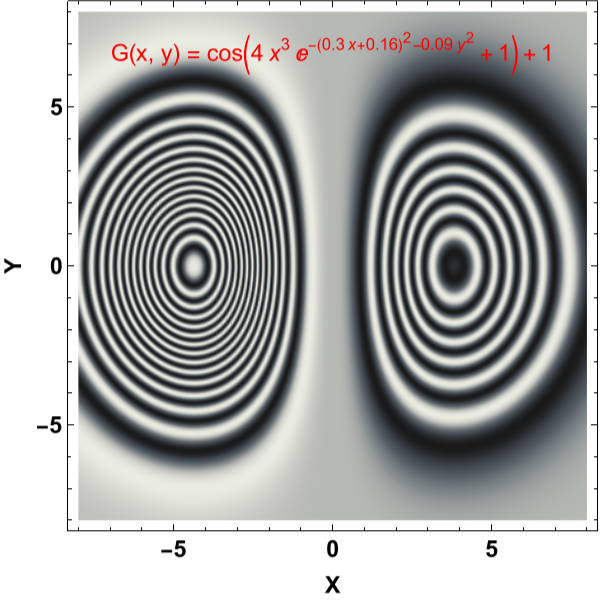
Process: Phase recovery from interferogram
Process: Phase recovery from interferogram
Obtaining the interferogram G from the seed phase ϕ is direct and straightforward. For the inverse process the 2D profile of the gray function G is an input, and 2D profile of the recovered phase is an output. In general, this output phase, denoted as φ, might be different from the seed phase ϕ.
1. Define and select G array slices
1. Define and select G array slices
xgynum[yn_]:=Map[G[#,yg[[yn]]]&,xg];(*returnsasinglex-sliceofG(x,y)forthegivenyindexynum*)
ygxnum[xn_]:=Map[G[xg[[xn]],#]&,yg];(*returnsasingley-sliceofG(x,y)forthegivenxindexxnum*)
Instead of operating on the full 2D G array we use a few G-slices. We slice G along the x-axes for given y-values and use them for phase recovery, while the single y-axis (for ) is used for determining the boundary condition of all phase profiles along the x-axes. Because the method works for both the x- and y-axes, see [1], the corresponding expressions for G, F, and |K| can be defined for both coordinates. Choosing a few slices for recovery saves computation resources and still delivers a reasonably accurate restored phase.
We chose to construct 21 equidistantly spaced G slices (remind that the G interval is [0,2]).
x=
x
min
2
K
We chose to construct 21 equidistantly spaced G slices (remind that the G interval is [0,2]).
selected=Range[1,Length[xg],20](*theseindicesareselectedandusedincoconstructionofG-slices*)
{1,21,41,61,81,101,121,141,161,181,201,221,241,261,281,301,321,341,361,381,401}
pxgl=Map[xgynum[#]&,selected];(*ThearrayofGx-slicesofG(x,y=fixed)definedbyselectedindices*)
pygl={ygxnum[1]};(*AsingleGy-sliceofG(x=xmin,y)-boundaryconditions*)
2. Construct F array slices from G array slices
2. Construct F array slices from G array slices
Compute the function F required to built the integrand K. For the given problem we have F=(G-A)/B, where A=B=1, corresponding to the case of the even illumination background and the noise free case. By definition F depends on the phase only, and the range of its values is [-1,1].
3. Interpolate F array slices along x- and y-axes
3. Interpolate F array slices along x- and y-axes
Up to this point, we have represented the input data as arrays, operating on them in a way that mimics the digital nature of real interferograms. From here onward, we will adopt Mathematica’s functional style of computation by interpolating the arrays into continuous functions. The interpolation is performed using high-order (8) splines.
Check its format: pxFl[[1]][1.3], first is an index of function, second is a coordinate
6. Compute phase
6. Compute phase
6.2 Integrate K for first y-slice (boundary condition for x-slices)
6.2 Integrate K for first y-slice (boundary condition for x-slices)
Computing the first y-slice profile. The inversion of the signs is indicated by “invy” (suggested values are provided in the section “Phase and its Visualization”). Set “invy” to 1 or -1 according to the interferogram boundary; if the correct value is not obvious, choose one at random. Then select “invx” to ensure the phase profile is consistent. After reconstruction, check whether the resulting phase profile is reasonable given the input; if it appears reversed, invert both “invy” and “invx”. Note that the signs of “invy” and “invx” are not necessarily the same.
Plot the obtained phase profile for first y-slice
6.5 Integrate K for each x-slice -- see Eq.(8)
6.5 Integrate K for each x-slice -- see Eq.(8)
Example of the computation of the x-slice profiles -- the first and third one. Note, the inversion of the signs is denoted by “invx”. (The suggested values for ‘invx’ are given in the section “Phase and its visualization”). Select 1 or -1 to match the interferogram boundary for G[x,0].
For each k-th x-slice we first find the value of the signed integral in (8) given by
RHSIntegral[KModx[k,x],x,Part[IntListx,k], invx*Part[signListx,k],dx]
RHSIntegral[KModx[k,x],x,Part[IntListx,k], invx*Part[signListx,k],dx]
For each k-th x-slice shift the phase values accordingly using the value Φ0y[k] given by the element phasePHI0vals[[k]].
6.6 Restore the phase surface
6.6 Restore the phase surface
Each of 21 elements corresponding to specific value y[k] of ‘yvals’ in ‘resxfinal’ is an array of pairs {x[i],ϕ[i,k]} and to restore the phase surface we have to replace each pair {x[i],ϕ[i,k]} by {x[i],y[k],ϕ[i,k]}.
Visualization of the restored phase φ.
Output: interferogram G with the seed ϕ and recovered φ phases
Output: interferogram G with the seed ϕ and recovered φ phases
CITE THIS NOTEBOOK
CITE THIS NOTEBOOK
Continuous recovery of phase from single interferogram
by Vyacheslav Berejnov and Boris Rubinstein
Wolfram Community, STAFF PICKS, March 30, 2026
https://community.wolfram.com/groups/-/m/t/3672004
by Vyacheslav Berejnov and Boris Rubinstein
Wolfram Community, STAFF PICKS, March 30, 2026
https://community.wolfram.com/groups/-/m/t/3672004