The purpose of this project is to critically examine and evaluate the claims put forth in the paper titled “Grover’s Algorithm Offers No Quantum Advantage”. The paper challenges the widely accepted notion that Grover’s algorithm, a quantum search algorithm, provides a significant speedup compared to classical algorithms. The project aims to investigate the validity of these claims and determine whether Grover’s algorithm truly offers no quantum advantage.
Introduction
Introduction
Within the realms of computational complexity theory a search problem is a particular type of computational problem that can be expressed as a binary relation . The essence of this problem lies in the pursuit of identifying a specific structure, denoted as "a," within an object called "b." To solve this problem, an algorithm is considered successful if it can ascertain the existence of at least one such structure and produce one occurrence of it as the output .
Algorithmic complexity refers to the evaluation of the time required for an algorithm to complete when provided with an input of size n . It is crucial for an algorithm to possess scalability, ensuring that it can deliver the result in a reasonable and finite time frame, even for significantly large values of n . To assess scalability, complexity is commonly analyzed asymptotically as n approaches infinity . Although complexity primarily focuses on time considerations, it is occasionally examined in terms of space requirements as well, which pertains to the algorithm' s memory utilization . By analyzing complexity, we gain insights into how algorithms perform and how their efficiency varies with input size .
Search problems play a fundamental role in various domains of computer science, ranging from data retrieval to optimization and decision - making . Optimization problems often involve finding the optimal configuration or arrangement of variables that minimize or maximize a given objective function. Search algorithms can iteratively explore the solution space, evaluating different combinations of variables, until an optimal solution is found. Examples of optimization problems include network routing, resource allocation, scheduling, and parameter tuning in machine learning algorithms. In decision-making contexts, search algorithms are employed to navigate through vast sets of options or alternatives to identify the most suitable choice based on specified criteria. This could involve evaluating different paths in a decision tree, searching for the best move in a game, or selecting the most optimal route in a navigation system.
Classical Search Algorithm
Classical Search Algorithm
The classical search algorithm, also known as exhaustive search, is a basic and widely employed method for finding a desired element within a given set . It involves sequentially examining each element of the set until a match is found or the entire set is exhausted . While simple and intuitive, the classical search algorithm can be computationally demanding, especially when dealing with large data sets . As the size of the input increases, the time required for the classical search algorithm to complete also grows linearly, resulting in a time complexity of , where n represents the size of the set . This linear growth limits its scalability and efficiency when dealing with significantly large search spaces .
O()
n
2
In the context of classical computing, when we have no prior information about the location of a specific target element in an unstructured set of N elements, we are required to examine each element individually in order to find the desired target.
For example, let’s consider a random integer from 1 to 10
In[]:=
ri=RandomInteger[{1,10}]
Out[]=
9
And a randomised list of integers from 1 to 10
In[]:=
rs=RandomSample[Table[x,{x,1,10}]]
Out[]=
{5,1,6,3,7,10,8,2,9,4}
The classical search algorithm operates by sequentially comparing the target element with each element in the list sequentially, starting from the beginning, until a match is found. Hence, the number of steps is at least equal to the position of the random integer in the list.
In[]:=
Position[rs,ri]
Out[]=
{{9}}
In[]:=
If[rs[[#]]==ri,Print[True],Print[False]]&/@Table[i,{i,1,10}];
False
False
False
False
False
False
False
False
True
False
After performing the search process 10 additional times, the position of the random integer within the list is as follows:
In[]:=
NumberSteps=Flatten[Table[Position[RandomSample[Table[x,{x,1,10}]],ri],10]]
Out[]=
{8,4,4,6,1,6,2,5,4,3}
Taking the average of the number of steps required
In[]:=
Mean[NumberSteps]//N
Out[]=
4.3
Theoretically, when searching for a specific element in a list of N elements, it takes an average of steps to locate the desired element. By repeating this process 10 more times, we can observe a consistent trend that supports this average.
N
2
In[]:=
FindElement[List_,Element_]:=Module[{p},p=Position[List,Element]]
In[]:=
r[x_]:=Table[Clear[r1];FindElement[r1,RandomChoice[r1=RandomInteger[{1,10},x]]],10]m=Table[N[Mean[Flatten[r[10]]]],10]Show[Plot[10/2,{xaxis,0,10},PlotLegends->"Theoretical prediction"],ListPlot[m,PlotStyle->Black],PlotRange->{0,10},AxesLabel->{"Trial Number","Number of steps"},ImageSize->Large]
Out[]=
{5.95455,5.16667,5.94444,6.04545,6.,5.14286,6.73333,5.55556,6.22222,4.45455}
Out[]=
Theoretical prediction |
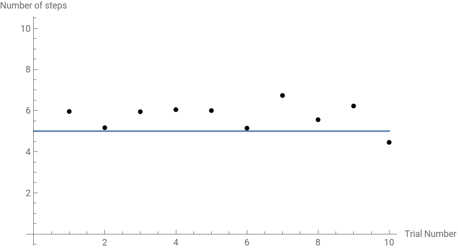
In classical computation, it is impossible to solve the search problem in fewer than O(N) evaluations. This is because, on average, one needs to examine approximately half of the elements in the search space.
Grover’s Algorithm
Grover’s Algorithm
In[]:=
PacletInstall["https://wolfr.am/DevWQCF",ForceVersionInstall->True]<<Wolfram`QuantumFramework`
Out[]=
PacletObject

Grover' s algorithm, a quantum search algorithm devised by Lov Grover, offers a significant improvement over classical search algorithms for certain types of search problems . By leveraging the principles of quantum computing, Grover' s algorithm achieves a remarkable speedup in the search process . It employs quantum superposition and interference to explore multiple elements of the search space simultaneously, significantly reducing the number of iterations required to find the desired solution . Unlike classical algorithms, Grover' s algorithm exhibits a quadratic speedup, with a time complexity of approximately . This exponential improvement makes Grover' s algorithm highly efficient for large search spaces .
O
n
2
The Grover algorithm is a quantum search algorithm that aims to efficiently find a specific element in an unsorted database. Through a careful design of iterations of a quantum system through an “oracle”, Grover’s algorithm can locate the target element with high probability using significantly fewer evaluations compared to classical approaches.
Consider selecting a bitstring of length “n” that requires a search operation.
In[]:=
n=5;
In[]:=
bitstring=StringJoin[ToString/@RandomInteger[{0,1},n]]
Out[]=
10101
The optimal number of iterations to find the target element is given by the expression where is the total number of elements in the search space. For the sake of clarity, we will consider 2 times of that optimal steps, to show changes in features we compute.
Floor
π
4
n
2
n
2
In[]:=
iter=2Floor[π/42^(n/2)]
Out[]=
8
Create a boolean function such that the chosen bitstring is the only solution.
In[]:=
vlist[bitstring_String]:=Module[{n=StringLength[bitstring],variables},variables=Table[If[StringTake[bitstring,{i,i}]=="0",Not[Symbol["v"<>ToString[i]]],Symbol["v"<>ToString[i]]],{i,n}]]
In[]:=
gneralGroverbf=Apply[And,vlist[bitstring]]
Out[]=
v1&&!v2&&v3&&!v4&&v5
The oracle in Grover’s algorithm is a vital component that facilitates the identification of the target state within the search space.
Quantum computers effectively boost the probability of identifying the desired item within a search space. This procedure involves amplifying the amplitude of the marked item while simultaneously reducing the amplitudes of the other items. As a result, the final state obtained after measurement will almost certainly correspond to the desired item. The procedure is done using two operators.
We shall consider the phase oracle (and not Boolean oracle).The phase operator changes the phase of the desired state while leaving the other states unchanged. It flips the sign of the amplitude of the marked item, effectively introducing a negative phase factor.
The diffusion operator performs a reflection operation about the average amplitude of the superposition. This reflection amplifies the amplitude of the target state while attenuating the amplitude of the non-target state. It effectively concentrates the amplitude around the target state, making it more distinguishable from the non-target states.
In[]:=
ga=N@QuantumCircuitOperator[{"GroverPhase",gneralGroverbf}];
In[]:=
ga["Diagram"]
Out[]=
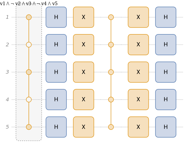
To initiate the procedure, the system begins in a state of uniform superposition. This superposition state provides an initial balance, ensuring that the search process begins without any bias towards a particular state. It also allows the algorithm to simultaneously evaluate multiple states in parallel, exploiting the power of quantum parallelism.
In[]:=
qs=N@QuantumState[{"UniformSuperposition",n}];
Iterate the process through the Grover oracle to increase the probability to find the target state.
In[]:=
gaSteps=NestList[ga,qs,2iter+1];
Given the state at any step, we can project it into subspace of the solution (yes, it is a bit cheating here, but it does not change the computation; the correct approach is to measure the qubits, and one will get the solution with a given probability).
In[]:=
gaW=QuantumOperator[QuantumState[bitstring]["Dagger"],{{},Range[n]}]
Out[]=
QuantumOperator

Now we illustrate it (note after 5 steps, one get the solution with the probability close to one)
Show the numerical values for probability of getting the solution:
Show the max value (as expected, close to one for the solution)
Number of iterations through the oracle required to maximize the probability of measuring the target element
The authors of the paper I am studying in this computational experiment, mentioned that throughout the process of each iteration, if one treats oracle and diffusion as one single package and apply them on state, the Entanglement Entropy shows an overall Bell-shape increase, with max at the optimal number of steps, but all values less than Log[2]
In order to find Entanglement Entropy, we consider all bipartitioning as follows:
Then search over them, and pick the max value of the entropy. For that purpose, we designed the following function. Note this it may take some time to compute, we are monitoring the entropy, as it is computed for each step (that is why we added Echo in the function)
A function to search for different bipartition and get max entropy
Compute the entanglement entropy at each step between the oracle calls for Grover’s Algorithm
Plot the entropy, for iteration of oracle and diffusion:
Oracle Described in the Paper: “Grover’s Algorithm Offers No Quantum Advantage”
Oracle Described in the Paper: “Grover’s Algorithm Offers No Quantum Advantage”
The authors present their findings by examining various aspects of Grover' s algorithm, such as the time complexity, space complexity, and the impact of noise and imperfections in real - world quantum systems . They argue that the theoretical quadratic speedup offered by Grover' s algorithm may not translate into significant practical advantages due to several factors, including the overhead associated with quantum computations, the limitations of quantum hardware, and the effects of decoherence and noise on quantum states . For that aim, they decompose oracle intro series of simpler controlled-gates, using ancillary qubits.
Construct the oracle described in the paper
Although not mentioned in the paper, we believe the authors have done the same decomposition, for the diffusion step, too
Now given the desired bit string, we can construct the overall circuit:
For this oracle , we have to start with 2n+1 qubits with the first n qubits in uniform superposition state and the next n qubits in state “0” and the last qubit in state “-“
Iterate the process through the oracle to increase the probability to find the target state .
Compute max entropy for above steps:
Now we categorize all entropy values as one big list, for all steps, and another one, for oracle-diffusion steps. Note that the whole idea was to look into steps within oracle or diffusion, since entropy increases during those steps, and using that feature (and not only superposition/parallelism).
Show them:
Quantum inspired Grover’s Algorithm
Quantum inspired Grover’s Algorithm
Generate oracle operator as in Eq.4
The original bitstring we considered
Test that above oracle is the same as the one we get automatically from PhaseOracle
Generate diffusion operator
Test it is the same as the one we get automatically from GroverPhaseDiffusion
Running through the steps of QiGA
Do the subtraction, as explained in Step-2 of page 6 in the paper:
Show it follows the expected formula:
MPS stands for Matrix Product State and refers to a tensor network representation of a quantum state . MPS provides a compact and efficient way to describe the quantum state of a system composed of multiple particles or qubits . In an MPS, the quantum state is represented as a product of tensors, where each tensor describes the state of an individual particle or qubit and its connections to neighboring particles . The key idea behind the MPS representation is that the state of each particle depends only on its local environment, allowing for an efficient and tractable description of the overall quantum state . The tensors in an MPS are typically chosen to have a low bond dimension, meaning that they have a small number of indices or parameters . This low bond dimension property enables efficient computations and manipulations of the quantum state.
Compute the MPS for each step
A function to compute the rank of MPS
Get the rank for all steps
Plot it together with entropies
Future Directions
Future Directions
Concluding Remarks
Concluding Remarks
In conclusion, this project successfully demonstrated the procedure outlined in the paper for a single target element search problem within Grover’s algorithm. However, it is important to acknowledge that due to time constraints and limitations in computational power, expanding the scope of the project to include a larger number of qubits and an increased number of solutions was not feasible. Nonetheless, this work serves as a valuable foundation for future investigations that can build upon the findings presented here and explore the potential of Grover’s algorithm in more complex search scenarios.
Keywords
Keywords
◼
Quantum Computing
◼
Complexity
◼
Grover’s Algorithm
◼
Quantum Entanglement Entropy
Acknowledgment
Acknowledgment
I am deeply grateful for Stephen Wolfram’s thought-provoking idea that have fueled my motivation throughout the course of this project. I express my sincere gratitude to Mads Bahrami, Nik Murzin and Shivam Sawarn for their exceptional explanations and valuable guidance. We thank the authors of the preprint for their valuable responses and clarifications regarding our inquiries. Their expertise and advice have been invaluable throughout my learning journey. Likewise, I would also like to thank Xerxes D. Arsiwalla for his continued support. I would like to extend my appreciation to all the fellow students in the physics track. Their presence and friendship have greatly contributed to making the summer school an incredibly enjoyable and enriching experience.
References
References
◼
arXiv:2303.11317v1 [quant-ph] 20 Mar 2023
CITE THIS NOTEBOOK
CITE THIS NOTEBOOK
Investigating the claims of "Grover's algorithm offers no quantum advantage"
by Suraj Vishwanath
Wolfram Community, STAFF PICKS, July 12, 2023
https://community.wolfram.com/groups/-/m/t/2958725
by Suraj Vishwanath
Wolfram Community, STAFF PICKS, July 12, 2023
https://community.wolfram.com/groups/-/m/t/2958725