Wolfram Cloud Document

ABSTRACT (original article): Spaces with negative curvature are particularly difficult to realize experimentally. In the original research article, we show how to emulate a discretized version of constant negatively curved space, a so called hyperbolic lattice, using an electric circuit network. We present static and dynamical methods which allowed us to characterize and verify the negative curvature in the implemented model. Our experiments showcase a versatile platform to emulate hyperbolic lattices in tabletop experiments, which can be utilized to explore propagation dynamics as well as to realize topological hyperbolic matter. This Wolfram Mathematica notebook showcases how we obtain the theoretical results, analyze the experimental data, and arrive at the conclusions stated in the article. CITATION (original article): Lenggenhager, P.M., Stegmaier, A., Upreti, L.K. et al. Simulating hyperbolic space on a circuit board. Nature Communications 13, 4373 (2022). DOI: https://doi.org/10.1038/s41467-022-32042-4
DATA & CODE: Patrick M. Lenggenhager (2021), https://doi.org/10.3929/ethz-b-000503548

Introduction

Curved spaces are usually associated with high-energy physics and cosmology. However, through the possibility of tabletop experiments emulating curved spaces and the interest in related synthetic matter, they have become relevant in condensed matter physics as well.

Spaces with negative curvature, however, are still difficult to realize experimentally. Here, we show how to emulate a discretized version of negatively curved space, a so called hyperbolic lattice, using an electric-circuit network. We present static and dynamical methods which allow us to characterize and verify the negative curvature in the implemented model. Both methods rely on the Laplace-Beltrami operator, the generalization of the Laplacian to curved spaces, and its manifestation in the lattice and ultimately in the electric-circuit network. This Wolfram Mathematica notebook reproduces the full theoretical and experimental analysis of the results presented in the original article.

Spectra of Euclidean and hyperbolic drums

We first study the spectrum and eigenmodes of a Euclidean and hyperbolic drum in the continuum. We use the Poincaré disk representation of the hyperbolic plane, which allows us to consider circular drums with radius

<=1

in both cases. The hyperbolic metric on the Poincaré disk is defined by the length element

-2

1-





.

Solution to the Laplace equation with Dirichlet boundary conditions

The eigenvalues and eigenmodes of the hyperbolic drum with

correspond to those of the Laplace-Beltrami operator, i.e., the generalization of the Laplacian to curved space:

1-



where

=∂∂

+∂∂



is the Laplacian on the Euclidean plane. A drum is fixed at the boundary, i.e., we have Dirichlet boundary conditions. Thus, the eigenvalues and eigenmodes of a Euclidean or hyperbolic drum are obtained by solving

with

=0,

where

g∈{E,H}

indicates the Euclidean and hyperbolic geometric, respectively,

n,l

are quantum numbers labeling the number of radial and angular zeroes of the eigenmode

with frequency

For comparison to the experiments, we set

In[]:=

r0=0.94;

Euclidean disk

In the Euclidean case, the solutions can be expressed as superpositions of Bessel functions:

(r,θ)=



(

lθ

where



(z)

are the Bessel functions of the first kind and

is the

(n+1)

zero of the function

k



(kr)

. In order to find these zeroes, we implement the following function:

In[]:=

ClearAll[AccumulateBesselZeroes]AccumulateBesselZeroes::usage="AccumulateBesselZeroes[n, test] produces a list of the zeroes x_0 of the Bessel function J_n(x) in ascending order up until test[x_0] returns False.";AccumulateBesselZeroes[n_,test_]:=Module[{res={},x0,k=1},x0=N@BesselJZero[n,k];While[test[x0],AppendTo[res,{n,x0}];k++;x0=N@BesselJZero[n,k];];res]AccumulateBesselZeroes::usage="AccumulateBesselZeroes[ test] produces a list of the zeroes x_0 of the Bessel function J_n(x) in ascending order and for ascending n up until test[x_0] returns False.";AccumulateBesselZeroes[test_]:=Module[{res={},x0,n=0,resn},x0=N@BesselJZero[n,1];If[test[x0],AppendTo[res,AccumulateBesselZeroes[n,test]];n++;While[test[x0],resn=AccumulateBesselZeroes[n,test];AppendTo[res,resn];AppendTo[res,{-#1,#2}&@@@resn];n++;x0=N@BesselJZero[n,1];]];Flatten[res,1]]

Calling it, we compute some zeroes in the form

{l,

}

In[]:=

(solE=SortBy[{#1,#2/r0,(#2/r0)^2}&@@@AccumulateBesselZeroes[#^2<1000&],#[[2]]&])//Short

Out[]//Short=

{{0,2.55833,6.54503},230,{12,33.468,1120.11}}

We plot the resulting energy vs. angular momentum dispersion (as in Fig. 2a of the article):

In[]:=

ListPlot[solE[[;;,{1,3}]],PlotRange{{0,20},{0,1000}},FrameTrue,FrameLabel{"l","λ"}]

Out[]=

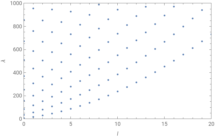
We observe clear branches of

, distinguished by different values of

. We also plot the eigenfunctions corresponding to the lowest six eigenvalues (see Fig. 1b):

Row[Module[{max},max=First@NMaximize[{Abs@BesselJ[#1,#2r],0≤r≤r0},r];Show[DensityPlot[Re[BesselJ[#1,#2Sqrt[x^2+y^2]]E^(#1ArcTan[x,y])],{x,y}∈Disk[{0,0},r0],PlotPoints50,ExclusionsNone,PlotRangeAll,ColorFunctionScalingFalse,ColorFunction(ColorData["BlueGreenYellow","ColorFunction"][Rescale[#,max{-1,1}]]&),FrameNone,FrameTicksNone,ImageSize->90],Graphics[{AbsoluteThickness[0.5],Black,Circle[{0,0},r0]}]]]&@@@Select[solE,#[[1]]≥0&][[;;6]]]

Poincaré disk

Similarly, the solutions to the Dirichlet problem in hyperbolic space can be expressed as superpositions of associated Legendre functions

(r,θ)=

(-1+

)

lθ

where

(z)

are the associated Legendre functions and

is the

(n+1)

zero of the function

k

(-1+k)

We implement the following function to numerically find these zeroes:

In[]:=

ClearAll[FindHyperbolicSolutions]FindHyperbolicSolutions::usage="FindHyperbolicSolutions::usage[m, x, kmax, δk] numerically finds zeroes of the function k -> LegendreP[1/2(-1+ k), m, x] in the range [0, kmax] with a resolution of δk.";Options[FindHyperbolicSolutions]={Tolerance7,Accuracy5};FindHyperbolicSolutions[m_,x_,kmax_,δk_,opts:OptionsPattern[{FindHyperbolicSolutions,FindRoot}]]:=Module[{res,tol=OptionValue[Tolerance],accuracy=OptionValue[Accuracy]},res=Table[FindRoot[Abs[LegendreP[1/2(-1+k),m,x]*LegendreP[1/2(-1+k),-m,x]]^20,{k,ki,ki,ki+δk},Evaluate@FilterRules[{opts},Options[FindRoot]]][[1]]/.Rule[a_,b_]Chop[b,10^-accuracy],{ki,Range[0,kmax,δk]}];res=DeleteDuplicatesBy[res,Round[#,10^-accuracy]&];res=Sort@Select[res,Im[#]0&&0≤#≤kmax&&Abs[LegendreP[1/2(-1+#),m,x]*LegendreP[1/2(-1+#),-m,x]]<10^-tol&]]

Evaluating it, gives:

In[]:=

(solH=SortBy[Flatten[ParallelTable[With[{sol={m,#,1+#^2}&/@Quiet@FindHyperbolicSolutions[m,(1+r0^2)/(1-r0^2),18,1]},If[m0,{sol},{sol,{-#1,#2,#3}&@@@sol}]],{m,0,20}],2],#[[3]]&])//Short

Out[]//Short=

{{0,1.46332,3.1413},262,{13,17.8046,318.004}}

which we plot again:

Hyperbolic lattices from tessellations

Euclidean tessellation

For the Euclidean drum, we consider a {3,6} tessellation, which we represent as the following graph (with coordinates assigned to the vertices):

Spectrum and eigenmodes

The graph represents a lattice if we interpret vertices as sites and edges and nearest-neighbor connections, which thereby define a metric. The graph Laplacian matrix then gives a lattice regularization of the continuum Laplace-Beltrami operator [Boettcher, I., Bienias, P., Belyansky, R., Kollár, A. J. & Gorshkov, A. V. Quantum simulation of hyperbolic space with circuit quantum electrodynamics: from graphs to geometry. Phys. Rev. A 102, 032208 (2020)]. In the long-wavelength-regime, eigenvalues and eigenvectors of the Laplacian matrix can be associated with their counterparts for the Laplace-Beltrami operator in the continuum, thereby giving us an approximation of the continuous drum.

We define the Laplacian matrix:

and diagonalize it, finding its eigenvalues and eigenvectors:

To be able to compare the eigenmodes on the lattice to those in the continuum, we first need to determine their angular momentum. To do that, we perform a Fourier transform in the angular coordinate:

The result is the angular momentum dispersion on the lattice (see Fig. 2b):

Hyperbolic tessellation

For the hyperbolic drum, we consider a {3,7} tessellation:

To visualize the lattice in the Poincaré disk, we need the following two functions.

Using that function, we implement the following function for visualizing a graph with vertices in the Poincaré disk such that the edges appear as geodesics:

For our case, we find:

where the red circle indicates the boundary of the drum, the unit circle is shown in blue, and three selected vertices (1,14, and 18) that will be relevant further below are highlighted in color.

Spectrum and eigenmodes

Analogously to the hyperbolic case, we construct the graph Laplacian

and determine its spectrum and eigenvectors:

While more sophisticated methods for determining the angular momentum on the Poincaré disk exist [D. M. Urwyler, P. M. Lenggenhager, I. Boettcher, R. Thomale, T. Neupert, and T. Bzdušek, Phys. Rev. Lett. 129, 246402 (2022)], here it is sufficient to proceed in the same way as for the Euclidean case, i.e., by performing a Fourier transform in the angular coordinate:

Again, we observe that the continuum dispersion is fairly well approximated. In particular, by comparing the result of the discretized Euclidean and hyperbolic drum, we reproduce the spectral reordering from the continuum:

The hyperbolic drum in a circuit: Simulations

To bring the Hyperbolic drum into physical reality, we realize the hyperbolic {3,7} Tessellation in the form of an electrical circuit network. In this, we can use measurements of voltages and currents to demonstrate the properties of hyperbolic geometry we discussed so far.

Constructing the circuit

First, we set up the circuit parameters

and add weights to the edges of the hyperbolic graphs to represent the capacitors placed there, with uniform random deviations according to part tolerances

To satisfy the discretized equivalent of Dirichlet boundary conditions, capacitors need to be added from the boundary nodes to ground, such that each circuit node is contacted by q=7 capacitors in total.

Impedances

We can measure the resonance spectrum of the circuit by looking at the impedances between the circuit nodes and ground. These impedances will peak whenever a resonance is present, and, importantly, this peak is also weighted by the local amplitude of the eigenvector corresponding to the resonance frequency. This way, impedance to ground can be thought of as a proxy for the local density of states. These impedances can be calculated as the diagonal elements of the inverted circuit-Laplacian. For comparison,we calculate the resonance frequencies of the ideal circuit (without tolerances or loss).

Note how the eigenfrequencies of the ideal circuit are proportional to the square roots of the inverted capacitance matrix, which is the hopping matrix. This means that the spectrum will appear inverted, with the lowest energy eigenmodes of the hyperbolic drum as the highest eigenfrequencies and well-separated from each other, so they can be easily identified in the spectrum as individual peaks.

Experiments

The circuit as described in the previous section was also realized in a real-world experiment. Here, we evaluate the recorded measurements.

Impedance measurements:

In order to determine the circuit’s resonant states, we performed impedance sweeps from several circuit nodes to ground. We import the measurement data using the command

dataZvsf = Association[(#1 -> Import[#2, "Table"][[3 ;;]]) & @@@ ({ToExpression@StringReplace[FileNameSplit[#][[-1]], RegularExpression["node(\\d+)\\.txt"] -> "$1"], #} & /@ FileNames[FileNameJoin[{NotebookDirectory[], "data", "experiments", "impedance", "node*"}]])];

For the purpose of this demonstration, we store the pre-processed data it in the notebook:

The data is given as an association with the key being the node number and the value a list with each element having the format {frequency [Hz], absolute value of complex impedance [Ohm], phase of complex impedance, real part of complex impedance [Ohm], imaginary part of complex impedance [Ohm]}.

We plot the impedance sweep of a few selected nodes (see figure above) together with the ideal theoretical eigenfrequencies,

Node 1 is the one at the center of the hyperbolic drum. From the n-l-quantization of the continuum, we expect that l ≠ 0 modes have a node at the center of the lattice, so their amplitude vanishes there and should make them vanish from the impedance spectrum. We can observe this effect in the measured sweep, where, going from high to low frequency, the impedance of node one shows two widely spaced peaks, whereas the other two nodes show intermediate peaks. Furthermore, by counting the peaks we see that the second l=0 mode appears as the sixth resonance frequency (not counting degeneracies). This confirms the hyperbolic nature of the circuit lattice due to the spectral reordering compared to the Euclidean disk, where the second l=0 mode is always in fourth position. This is caused by the shallower angular dispersion of hyperbolic space due to the comparatively larger radius of circles in it.

Eigenmodes

Furthermore, we resolve the eigenmodes of the circuit by exciting it with an AC current at the respective resonance frequency, fed into a node with high expected overlap with the eigenmode. In our original notebook, this was done by

ClearAll[ImportVoltageProfile]
ImportVoltageProfile::usage = "ImportVoltageProfile[measid] imports the voltage profile data for the measurement with id measid.";
ImportVoltageProfile[measid_] := Module[{
data = Import[FileNameJoin[{NotebookDirectory[], "data", "experiments", "voltage_profile", ToString@StringForm["meas_`1`.txt", measid]}], "Table"][[1]],
len, dataV, dataI
},
len = Length[data]/4;
data = (#1 + I #2) & @@@ Partition[data, 2];
dataV = data[[;; len]];
dataI = data[[len + 1 ;;]];
<|"V" -> dataV, "I" -> dataI|>
]
dataModes = (ImportVoltageProfile@#[[1, 1]] & /@ GroupBy[#, #[[3]] &]) & /@ GroupBy[SortBy[Import[FileNameJoin[{NotebookDirectory[], "data", "experiments", "voltage_profile", "input.txt"}], "CSV"][[2 ;;]], {-#[[2]] &, #[[3]] &}], #[[2]] &];*

Here, we again have the pre-processed data ready in the notebook

The data is given as a nested association with the key of the first level being the excitation frequency, the one of the second the excitation node, and the third the measured quantity, i . e ., "V" for voltage and "I" for current . Finally, the value is a list of complex - valued data points, each entry corresponding to a node in the circuit and represented by the graph gH .

We Plot a selection of six eigenmodes

Using the plot functions

From left to right, these are the eigenmodes associated with quantum numbers (n,l) = (1,0), (1,1) , (1,2), /1,3), (1,4) and (2,0). They correspond to the six highest resonance frequencies, not counting degeneracy. From the shape and symmetries of the plotted modes, we visually confirm our earlier evaluation, which is that the radially symmetrical (2,0) mode appears in sixth position.

Time - Resolved Measurement

In our final measurement, we observe the propagation of a pulse excitation in the lattice. According to its hyperbolic geometry, one expects wave fronts in the shape of hyperbolic circles to emerge in the initial propagation of the pulse (i.e. before waves reflected from the boundary dominate the signal).
We imported the measured signals using

dataPulse = Import[FileNameJoin[{NotebookDirectory[], "data", "experiments", "pulse", ToString@StringForm["Node_`1`_`2`Hz.txt", 31, 1/2 10^6]}], "Table"][[3 ;;]];

dataPulse definition is available in an attached notebook below in form of input cell.

Each entry of dataPulse corresponds to a time step of the recorded signal, and is a list containing time, Voltage of node 1, its absolute and argument based on the analytic signal and the same for all other nodes in order.

The circuit is excited by a current pulse fed into node 31, as shown below:

We can visualize the spreading of wave fronts by plotting the phase of the signal, which was obtained using the Hilbert transform in pre-processing.

The plot shows the concentric hyperbolic circles around the node of excitation. This exemplifies that the circular wave-fronts propagate through the circuit network according to the underlying hyperbolic metric implied by the lattice. If we look at the phase fronts over time, we see that they converge towards the point of excitation instead of diverging away from it. This is due to the left-handed dispersion described before, where phase and group velocity have opposite sign. At later times we see that the reflected signal starts to dominate and the concentric wave-fronts disappear.

Conclusion

Our experiments showcase a versatile platform for emulating hyperbolic lattices in tabletop experiments, which can be utilized to explore dynamics as well as to realize topological hyperbolic matter . Future developments in this field have the potential to advance our understanding of physics in curved spaces and to provide new perspectives on problems in condensed matter theory, high - energy physics and cosmology.

CITE THIS NOTEBOOK

Simulating hyperbolic space on a circuit board
by Patrick M. Lenggenhager
Wolfram Community, STAFF PICKS, November 8, 2023
https://community.wolfram.com/groups/-/m/t/3062320