In this notebook we explore the properties of random quantum circuits. Random quantum circuits can be derived in a variety of ways. The most straightforward way is to create a unitary matrix of a desired dimension (in this case where is the number of qubits in the system), then turn that matrix into an operator on the circuit. However, this process is not straightforward to implement on a quantum device, since the unitary matrix must be broken down into operations that can be implemented on quantum hardware.
n
2
n
For a randomly generated unitary matrix, qiskit supports circuit decomposition and transpilation, two related operations that decompose a circuit into simpler, implementable operations. However, these operations are computationally expensive and, even for circuits with small numbers of qubits, result in circuits of very high depth. Below is a plot of the depth of the transpiled/decomposed circuits for various qubit unitary operators.
n
In[]:=
transpiled={{2,7},{3,41},{4,197},{5,869},{6,3653},{7,14981},{8,60677}};decomposed={{2,7},{3,30},{4,175},{5,815},{6,3503},{7,14511},{8,59055}};ListPlot[{transpiled,decomposed},PlotLabel->"Circuit Depth for the Qiskit Implementation of Random Unitary Matrices",Joined->True,PlotLegends->{"Transpiled","Decomposed"},AxesLabel->{"Qubits","Circuit Depth"},ImageSize->Large]
Out[]=
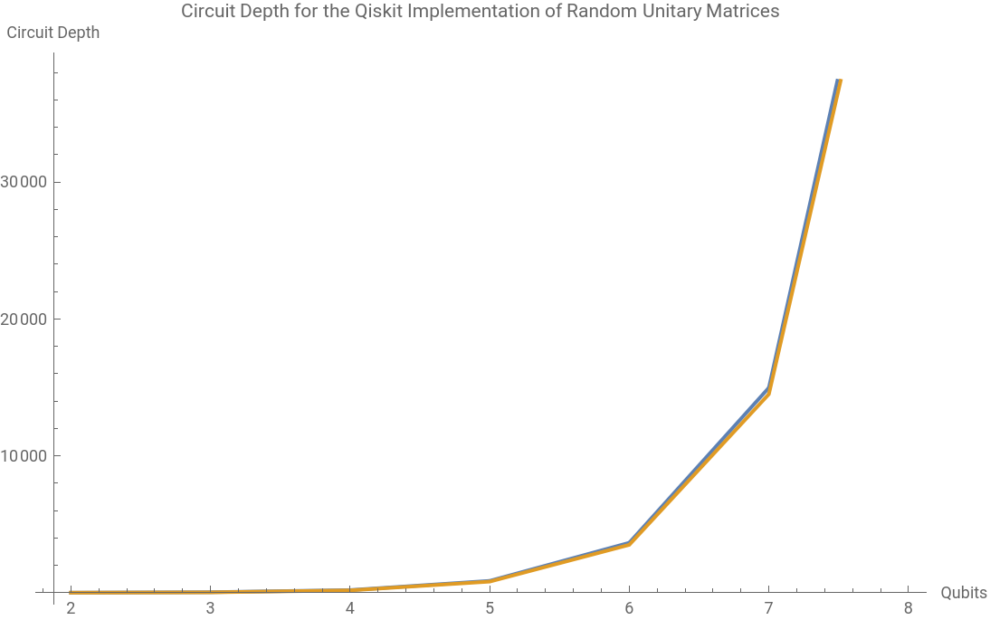


For current quantum computers, circuit depths beyond that of the 3 qubit decomposed depth of 30 are extremely difficult to implement, while circuit depths like those of the 5 qubit decomposition, 815, are next to impossible to implement.
This project explores the properties of random unitary matrices and an alternative method for generating random circuits that I created. First we will explore some properties of random unitary matrices and the quantum circuits that result.
Understanding Some Properties of Random Unitary Matrices
Understanding Some Properties of Random Unitary Matrices
The distribution of all random unitary matrices of dimension is given in Mathematica by the function CircularUnitaryMatrixDistribution[n]. A random 4x4 unitary matrix is generated with the code below:
n
In[]:=
SeedRandom[321];RandomVariate[CircularUnitaryMatrixDistribution[4]]//MatrixForm
Out[]//MatrixForm=
-0.0854648-0.237646 | -0.462773-0.586205 | 0.187961+0.195956 | 0.525325+0.1695 |
0.269077-0.147101 | -0.0282404-0.314087 | -0.225682-0.854159 | 0.050619-0.153064 |
0.576759-0.419696 | -0.290729+0.447802 | 0.130865-0.0152681 | -0.0333534+0.433225 |
0.563674-0.125122 | 0.238204-0.0310754 | -0.0713887+0.351137 | 0.305585-0.622201 |
Magnitudes of Random Unitary Matrix Elements
Magnitudes of Random Unitary Matrix Elements
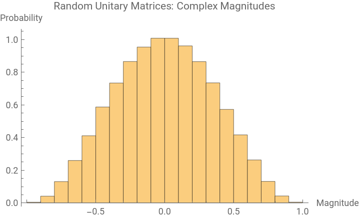
Let’s explore some properties of these random unitary matrices. First, let’s consider the distribution of the magnitude of each of the elements of the matrix. Here we generate a large set of these matrices and see what the distribution is. Note that we’ll be working with 4x4 unitary matrices, which corresponds to a 2 qubit system, but all of these calculations can be adjusted by changing the dimension of the matrix.
SeedRandom[123];(*Takethefirstcolumnofeachmatrix*)randomUnitaryList=RandomVariate[CircularUnitaryMatrixDistribution[4],40000];randomUnitaryMatrixElementList=Flatten[randomUnitaryList];randomUnitaryImaginaryElements=Im/@randomUnitaryMatrixElementList;randomUnitaryRealElements=Re/@randomUnitaryMatrixElementList;
Histogram[randomUnitaryImaginaryElements,Automatic,"ProbabilityDensity",PlotLabel->"Random Unitary Matrices: Imaginary Magnitudes",AxesLabel->{"Magnitude","Probability"}]
Out[]=
In[]:=
Histogram[randomUnitaryRealElements,Automatic,"ProbabilityDensity",PlotLabel->"Random Unitary Matrices: Real Magnitudes",AxesLabel->{"Magnitude","Probability"}]
Out[]=
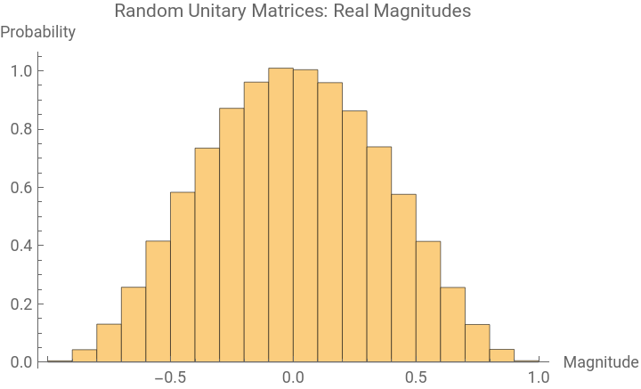
Notice that the distributions look quite a bit like normal distributions. We can test this informal assumption with a function called DistributionFitTest, which tests the data to see if it follows a normal distribution with some mean and variance. A value returned that is close to 0 tells us that it is unlikely that the data is normally distributed.
DistributionFitTest[randomUnitaryImaginaryElements]
Out[]=
0
In[]:=
DistributionFitTest[randomUnitaryRealElements]
Out[]=
0
Since this data fails to play nicely, let’s try FindDistribution, which looks for the distribution from the data
FindDistribution[randomUnitaryImaginaryElements]
Out[]=
MixtureDistribution[{0.578626,0.421374},{NormalDistribution[-0.186927,0.294402],NormalDistribution[0.285319,0.28232]}]
In[]:=
FindDistribution[randomUnitaryRealElements]
Out[]=
MixtureDistribution[{0.491203,0.508797},{NormalDistribution[-0.227759,0.281008],NormalDistribution[0.248293,0.282724]}]
This isn’t particularly satisfying either, since any distribution can be expressed as a mixture of two distributions. Not knowing the difficulty of finding the underlying distribution, we will examine a bit more. As we will see later, not knowing the distribution of the values will not be a problem for further analysis.
One important disclaimer is this, which applies to all of the tests in this project: just because we couldn’t guess or DistributionFitTest couldn’t guess the distribution doesn’t mean that there isn’t a closed form available. Hopefully one will be found and we can confirm it with the proper statistical methods.
One important disclaimer is this, which applies to all of the tests in this project: just because we couldn’t guess or DistributionFitTest couldn’t guess the distribution doesn’t mean that there isn’t a closed form available. Hopefully one will be found and we can confirm it with the proper statistical methods.
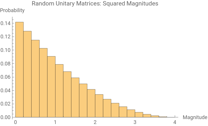
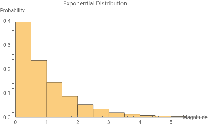
We can examine one more aspect of the matrices, the distribution of the magnitudes squared of the matrix elements. It faces similar problems to the real and imaginary parts, looking a lot like a scaled exponential distribution without actually being a scaled exponential distribution. The following two plots compare the two, and we can see their similarity and differences, with a proper statistical test putting a final nail in the coffin.
In[]:=
randomUnitaryElementMagnitudes=Abs[#]^2&/@randomUnitaryMatrixElementList;Histogram[randomUnitaryElementMagnitudes*4,20,"Probability",PlotLabel->"Random Unitary Matrices: Squared Magnitudes",AxesLabel->{"Magnitude","Probability"}]
Out[]=
In[]:=
Histogram[RandomVariate[ExponentialDistribution[4],40000]*4,20,"Probability",PlotLabel->"Exponential Distribution",AxesLabel->{"Magnitude","Probability"}]
Out[]=
In[]:=
FindDistribution[randomUnitaryElementMagnitudes]
Out[]=
MixtureDistribution[{0.649637,0.350363},{HalfNormalDistribution[7.10893],GammaDistribution[8.635,0.0532405]}]
In[]:=
DistributionFitTest[randomUnitaryElementMagnitudes/4,ExponentialDistribution[1]]
Out[]=
3.8114×
-13
10
Once again, not ideal, but it’s not the end of the story. We’ll continue our exploration in the next subsection with another matrix property.
Distribution of Eigenvalue Phases
Distribution of Eigenvalue Phases
We’ll continue our exploration by considering the phases of the eigenvalues of the unitary matrices. For context, the eigenvalues of unitary matrices are of the form where is a real number in . If this distribution is uniform, we should see a smear over the interval
iϕ
e
ϕ
[-π,π)
[-π,π)
In[]:=
SeedRandom[234];randomUnitaryList=RandomVariate[CircularUnitaryMatrixDistribution[4],10000];randomUnitaryEigenvalues=Flatten[Eigenvalues/@randomUnitaryList];randomUnitaryEVPhases=Arg/@randomUnitaryEigenvalues;
In[]:=
Histogram[randomUnitaryEVPhases,Automatic,"ProbabilityDensity",PlotLabel->"Distribution of Eigenvalue Phases for Random Unitary Matrices",AxesLabel->{"Phase","Probability Density"},ImageSize->Large]
Let’s do a test for uniform distribution. Hopefully this will actually confirm our suspicions
Random Unitary Matrices as Quantum Operators
Random Unitary Matrices as Quantum Operators
We can explore the behavior of these random unitary matrices as operators on quantum states, i.e. as unitary operators in a quantum computer. We can create a quantum circuit and apply a random unitary matrix as an operator. One property of interest is the entanglement produced by this random unitary operator. This can be analyzed with the entanglement entropy, which the Wolfram QuantumFramework has a built-in capacity to calculate.
We can do the same exploration with this output; we can try and find the distribution associated with the entanglement entropy. I’ve taken the liberty of overlaying a plot of the entanglement entropy with a plot of the fitted distribution
Once again we’re faced with a similar situation: the distribution is just a little off from what we’re looking for. It fits visually but fails the actual statistical test. However, these three metrics (matrix element magnitude, eigenvalue phases, and entanglement entropy) will serve as metrics against which we can test our random circuit generator.
Introducing Our randomUniversalCircuit Function
Introducing Our randomUniversalCircuit Function
Quantum circuits can span any numbers of qubits, and many specialized, named quantum gates with specific functions, uses, and properties have been identified. However, it has been proven that any quantum circuit, and, indeed, any unitary operator, can be represented by sets of gates called “universal quantum gates”. As was mentioned in the introduction, this process of breaking down a random unitary matrix (i.e. a quantum circuit operator) into these universal/implementable gates is quite expensive. Here, we go the other way, and take a set of two-qubit universal quantum gates that are easily implementable and try to build up a random unitary operator. This has the advantage of not needing to be broken down into a gigantic circuit: the circuit has already been built from the random selections.
Here is the code for my function:
Let’s generate a random circuit and look at the diagram, matrix form, output state, and probability plot for a 3 qubit system
Analyzing randomUniversalCircuit vs Random Unitary Matrices
Analyzing randomUniversalCircuit vs Random Unitary Matrices
We can generate the matrix representations for these random circuits and analyze them just the way we did with the output from the CircularUnitaryMatrixDistribution function in the previous section. For sake of simplicity and computational ease, we work first with 2-qubit examples. Later we will touch on higher-qubit systems.
randomUniversalCircuit and Matrix Element Magnitudes
randomUniversalCircuit and Matrix Element Magnitudes
Let’s first examine the magnitude of matrix elements with the same approach as before. Be careful running this code, it will take a while if you stick with a table of 800 random circuits (ironically, creating the random circuit takes much longer on classical computers than creating the unitary matrices, the opposite of the case for quantum computers).
Once again, finding the analytic distribution seems unsuccessful. However, we can approach this a different way: we can compare the distribution of results from our “oracle”--in this case, the distribution from the 640,000 data points done earlier--to the results here and see how close they are. Below we create the oracle distribution, then compare the difference of the two, normalizing for the difference in sample size.
This is excellent news: the distributions only differ by 0.01 at any bin at most, and only by 0.04 overall. One has to be careful to draw too many conclusions from this, but we can safely assume the data is similarly distributed in this situation (number of qubits, circuit depth, and CNOT ratio).
Since this is, of course, not rigorous, check out the “Further Work” section for a brief discussion of available options
Since this is, of course, not rigorous, check out the “Further Work” section for a brief discussion of available options
randomUniversalCircuit Eigenvalue Distribution
randomUniversalCircuit Eigenvalue Distribution
Let’s now analyze the distribution of eigenvalues. Since we know we’re looking for a uniform distribution, this will be easy, with no need to compare the oracle to the new data.
We can, of course, run the same test on this data to see if it is uniformly distributed.
And, once again, we’re not left disappointed. The high p-value allows us to fail to reject the null hypothesis that the data is uniformly distributed.
randomUniversalCircuits and Entanglement Entropy
randomUniversalCircuits and Entanglement Entropy
We can also look at the effect of these circuits on a quantum state, namely the entanglement entropy, just like the previous unitary operators.
Unfortunately this also fails the statistical test and appears to not really fit the result of FindDistribution
However, we can employ a similar tactic to the magnitudes and examine a comparison to the oracle.
Here we see promising results, with differences between the two distributions hitting a maximum of 0.035 and having a total difference of 0.15. This should tell us that we’re on the right track
Conclusions and Further Work
Conclusions and Further Work
We have here essentially introduced a new way to generate random quantum circuits that has a distinct advantage: not requiring decomposition, an expensive and circuit-depth producing process. Upon creating this new method of generating random quantum circuits, we must make sure they are actually generating random unitary matrices that correspond to random quantum circuits. There exists a myriad of matrix properties that can be analyzed and another myriad of properties that quantum circuits can have, but there is no way to take a data set of unitary matrices and test whether or not they uniformly sample from the space of all unitary matrices.
Here we have taken three prominent necessary conditions for randomness (distribution of matrix elements, eigenvalues, and induced entanglement entropy) and shown comparable results in the 2 qubit case for all three properties. This is hopefully the start of a promising alternative to the standard methods of random quantum circuit generation.
Further work centers around expanding the computational experiments on the function parameters, e.g. varying the number of qubits, circuit depth, and CNOT ratios and on expanding and formalizing the tests of randomness. Methods like the KullbackLeiblerDivergence to analyze the similarity of any probability distribution and the Wasserstein metric for the distance between two probability distributions are promising possibilities to formalize the “oracle” comparison that was performed in this experiment. Further analyzing the final state vector and the resulting measured distribution are also promising areas of research.
Here we have taken three prominent necessary conditions for randomness (distribution of matrix elements, eigenvalues, and induced entanglement entropy) and shown comparable results in the 2 qubit case for all three properties. This is hopefully the start of a promising alternative to the standard methods of random quantum circuit generation.
Further work centers around expanding the computational experiments on the function parameters, e.g. varying the number of qubits, circuit depth, and CNOT ratios and on expanding and formalizing the tests of randomness. Methods like the KullbackLeiblerDivergence to analyze the similarity of any probability distribution and the Wasserstein metric for the distance between two probability distributions are promising possibilities to formalize the “oracle” comparison that was performed in this experiment. Further analyzing the final state vector and the resulting measured distribution are also promising areas of research.
CITE THIS NOTEBOOK
CITE THIS NOTEBOOK
Exploring random quantum circuits without unitary matrix decomposition
by Charles Woodrum
Wolfram Community, STAFF PICKS, July 13, 2023
https://community.wolfram.com/groups/-/m/t/2959853
by Charles Woodrum
Wolfram Community, STAFF PICKS, July 13, 2023
https://community.wolfram.com/groups/-/m/t/2959853