Dimensions are most commonly known in terms of the degrees of freedom (number of coordinates) in the real space. It becomes obvious from that that we perceive our universe in four dimensions: 3 spatial dimensions and one temporal dimensions. This study will only concern itself with spatial dimensions. So, from now, ‘dimensions’ will only refer to spatial dimensions. In the Wolfram model, dimensions are defined with respect to the volume (measured as the number of nodes within a particular radius from a central node). It has then been observed that the volume increases roughly as r^d where r is the radius and d is the dimension [1]. This study will look at how dimensions evolve in the Wolfram model for certain rules, its relationship to the universe and how this definition of dimensions work out.
We start with a simple model as such:
Verification of method with a simple rule
Verification of method with a simple rule
In[]:=
WolframModel[{{{1,2}}{{1,1},{3,1}}},{{1,2}},6,"FinalStatePlot"]
Out[]=
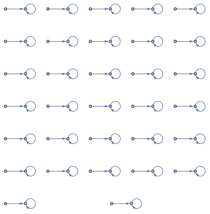
For this rule, we see that the distribution of dimensions (given by a histogram) looks like:
In[]:=
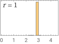
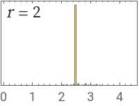
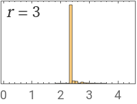
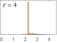
FullLDList[g_]:=N[ResourceFunction["LogDifferences"]/@HypergraphNeighborhoodVolumes[g,All,Automatic]];Module[{r=1},Histogram[#,PlotRange{{0,4.5},Automatic},FrameTrue,FrameTicks{Automatic,None},ImageSizeTiny,EpilogText[Style[Row[{Style["r",Italic],StringTemplate[" = ``"][r++]}],Directive[FontSize12,GrayLevel[0.2],FontFamily"Source Serif Pro"]],Scaled[{0,1}],{-1.3,1.1}]]&/@Transpose[Values[FullLDList[WolframModel[{{{1,2}}{{1,1},{3,1}}},{{1,2}},6,"FinalState"]]]]]
Out[]=
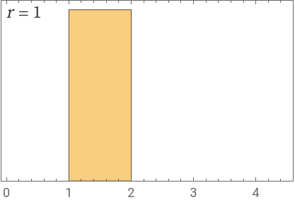
This shows that the hypergraph is always 1- dimensional. This makes sense since the maximum graph distance of between two connected nodes is always 1 and so the notion of dimensions described by the Wolfram models work. Let’s now investigate another rule.
Investigating with a complex rule: Part 1.1
Investigating with a complex rule: Part 1.1
In[]:=
WolframModel[{{{1,1,2},{2,3,4}}{{5,5,4},{1,5,4},{2,5,3}}},{{1,1,1},{1,1,1}},900,"FinalStatePlot"]
Out[]=
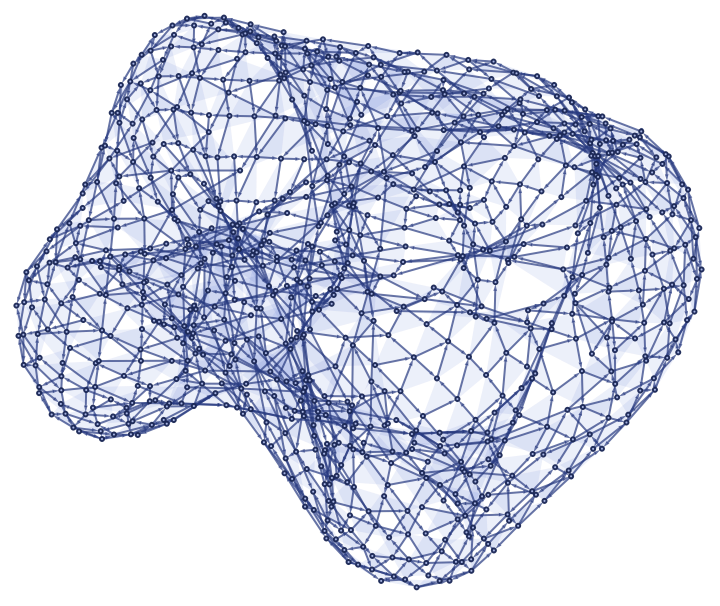
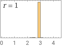
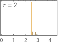
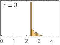
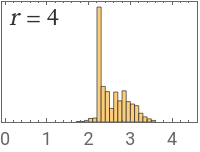
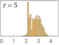
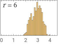
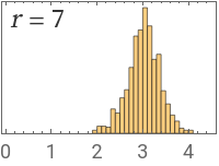
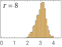
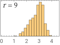
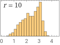
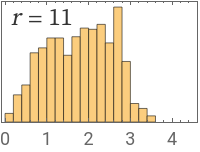
For 900 evolutions of this hypergraph, we see the distribution of dimensions to be:
In[]:=
FullLDList[g_]:=N[ResourceFunction["LogDifferences"]/@HypergraphNeighborhoodVolumes[g,All,Automatic]];Module[{r=1},Histogram[#,PlotRange{{0,4.5},Automatic},FrameTrue,FrameTicks{Automatic,None},ImageSizeTiny,EpilogText[Style[Row[{Style["r",Italic],StringTemplate[" = ``"][r++]}],Directive[FontSize12,GrayLevel[0.2],FontFamily"Source Serif Pro"]],Scaled[{0,1}],{-1.3,1.1}]]&/@Transpose[Values[FullLDList[WolframModel[{{{1,1,2},{2,3,4}}{{5,5,4},{1,5,4},{2,5,3}}},{{1,1,1},{1,1,1}},900,"FinalState"]]]]]
Out[]=
,
,
,
,
,
,
,
,
,
,
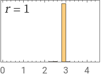
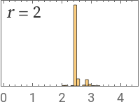
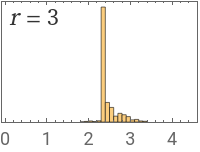
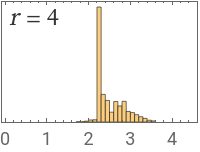
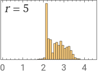
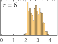
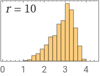
For 1200 evolutions, this changes to:
In[]:=
FullLDList[g_]:=N[ResourceFunction["LogDifferences"]/@HypergraphNeighborhoodVolumes[g,All,Automatic]];Module[{r=1},Histogram[#,PlotRange{{0,4.5},Automatic},FrameTrue,FrameTicks{Automatic,None},ImageSizeTiny,EpilogText[Style[Row[{Style["r",Italic],StringTemplate[" = ``"][r++]}],Directive[FontSize12,GrayLevel[0.2],FontFamily"Source Serif Pro"]],Scaled[{0,1}],{-1.3,1.1}]]&/@Transpose[Values[FullLDList[WolframModel[{{{1,1,2},{2,3,4}}{{5,5,4},{1,5,4},{2,5,3}}},{{1,1,1},{1,1,1}},1200,"FinalState"]]]]]
Out[]=
,
,
,
,
,
,
,
,
,
,
,
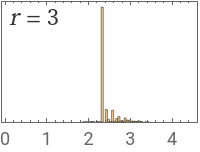
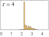
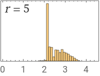
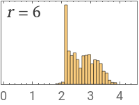
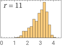
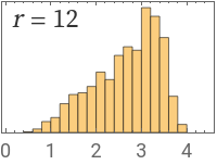
For 1600 evolution steps, the plots are now:
In[]:=
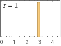
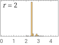
FullLDList[g_]:=N[ResourceFunction["LogDifferences"]/@HypergraphNeighborhoodVolumes[g,All,Automatic]];Module[{r=1},Histogram[#,PlotRange{{0,4.5},Automatic},FrameTrue,FrameTicks{Automatic,None},ImageSizeTiny,EpilogText[Style[Row[{Style["r",Italic],StringTemplate[" = ``"][r++]}],Directive[FontSize12,GrayLevel[0.2],FontFamily"Source Serif Pro"]],Scaled[{0,1}],{-1.3,1.1}]]&/@Transpose[Values[FullLDList[WolframModel[{{{1,1,2},{2,3,4}}{{5,5,4},{1,5,4},{2,5,3}}},{{1,1,1},{1,1,1}},1600,"FinalState"]]]]]
Out[]=
,
,
,
,
,
,
,
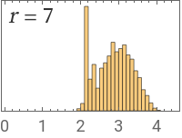
,
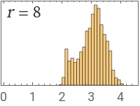
,
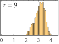
,
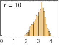
,
,
,
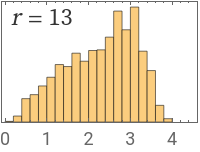
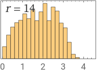
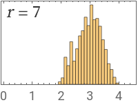
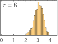
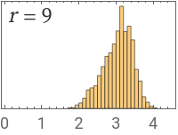
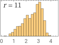
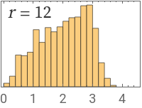
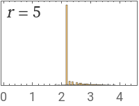
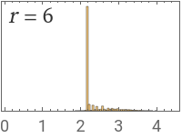
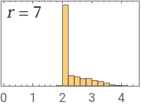
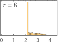
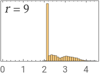
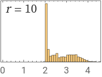
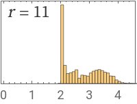
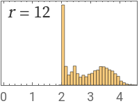
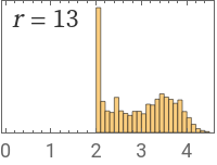
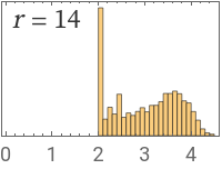
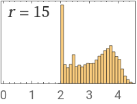
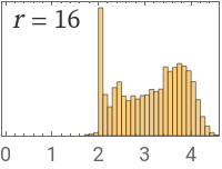
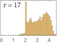
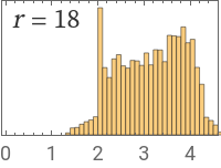
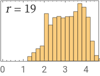
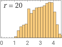
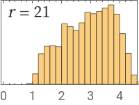
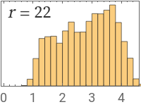
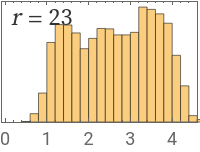
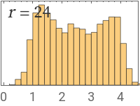
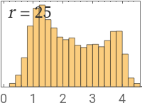
Notice how the maximum radius is increasing with more evolution steps. That is to be expected since more nodes are formed at further distance at each evolution. Let’s now inspect how the distributions change at each scale, that is, for a particular radius. We notice that the distribution keeps having a finer peak at a certain dimension for each radius with increased number of steps. One might form a conjecture that the distributions are Gaussian and the variance refers to the curvature of space e.g. near a black hole. But we can see that that is not the case for this rule. For instance, when we run it for 8000 steps, the distributions (focus on r=7,8,9, which were most ‘normal’ for <1600 steps) become to be:
In[]:=
FullLDList[g_]:=N[ResourceFunction["LogDifferences"]/@HypergraphNeighborhoodVolumes[g,All,Automatic]];Module[{r=1},Histogram[#,PlotRange{{0,4.5},Automatic},FrameTrue,FrameTicks{Automatic,None},ImageSizeTiny,EpilogText[Style[Row[{Style["r",Italic],StringTemplate[" = ``"][r++]}],Directive[FontSize12,GrayLevel[0.2],FontFamily"Source Serif Pro"]],Scaled[{0,1}],{-1.3,1.1}]]&/@Transpose[Values[FullLDList[WolframModel[{{{1,1,2},{2,3,4}}{{5,5,4},{1,5,4},{2,5,3}}},{{1,1,1},{1,1,1}},8000,"FinalState"]]]]]
Out[]=
,
,
,
,
,
,
,
,
,
,
,
,
,
,
,
,
,
,
,
,
,
,
,
,
,
,
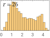
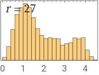
We find that none of the distributions show central tendency anymore. This trend of not having any such trend follows for any higher number of evolutions for this rule. Let’s check if this is unique to this particular rule.
Investigating with a complex rule: Part 2.1
Investigating with a complex rule: Part 2.1
In[]:=
WolframModel[{{{1,2},{1,3},{1,4}}{{1,1},{5,1},{5,2},{3,5},{4,3}}},{{1,1},{1,1},{1,1}},25,"FinalStatePlot"]
Out[]=
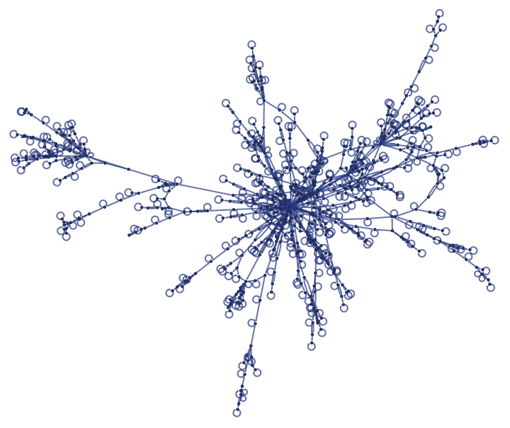
For 25 evolution steps of this rule, we find,
For 30 steps, the distribution becomes,
Just like the previous rule, we see that here as well the distributions are quite irregular. But one common feature across all the distributions for both rules for any specific radius is that the peak dimension of the distribution decreases with more steps. That is, the average dimensionality decreases as the distance between the nodes increases with more evolution steps. To understand this better, let’s see the effect on average dimensionality for each radius with respect to distance between nodes.
Investigating with a complex rule: Part 1.2
Investigating with a complex rule: Part 1.2
For the first complex rule used before, we look at a series of difference in dimensionality vs hypergraph distance plots for each radius (for 900 evolution steps at first). We notice that the difference in dimensionality does decrease over time for radius equal to 1 to 5. But this trend also doesn’t follow for higher radii.
If we carry out the same process for 1200 steps of the rule, we see,
Even now, the trend is not decreasing as expected. Let’s then look at the second rule.
Investigating with a complex rule: Part 2.2
Investigating with a complex rule: Part 2.2
Following the same method as before, for 25 steps of the second rule, we notice the following trend,
That is, the plots did not really decrease with increasing radii.
Despite the irregularity, we do see some ‘regularity’ in terms of how the graphs fluctuate. One potential explanation might be about how there were a lot of quantum fluctuations in the period of inflation. In that case, the fluctuations should stabilize over time. Let’s investigate that.
The plots here are looking at the difference in dimensionality with respect to hypergraph distance for a certain radius for a number of evolution steps of a Wolfram model. Here, we see that the plots are tending towards certain shape for a generally increasing scale. Let’s see the same for another rule.
Here, the trend isn’t that stabilizing anymore. But the number of peaks is roughly constant. So, we now know that there exists certain rules for which we observe a lot of initial fluctuations and stability later on. This can be a property that can be used as a litmus test for any rule that can represent our universe.
Discussion and potential interpretation
Discussion and potential interpretation
There can be two possible reasons why the plots are not behaving as expected. One can be that the rules used for the investigation were arbitrarily like this and there might be some other rule which might behave as expected. The properties required for the rule to behave such way is not clear and can be investigated. The other potential issue might be with the definition of dimensions in the Wolfram model. Georg Cantor showed that the coordinate definition of dimensions are not homeomorphic and hence leads to a paradox [2]. The case might be similar for the volume based definition and it needs to be checked. Another issue can be that the effect of the non-leading terms, which the volume based definition ignores, is large enough for the dimension estimation to be wrong. Also, such definition seems quite Euclidean and can break down when space is curved. Potential alternatives for the volume definition of dimensions are available. One such prominent alternative is the Spectral dimension, which deals with dimensions of spectral structures [3]. This should possibly be reasonably implemented in the Wolfram model and the same procedure as above can be carried out.
Keywords
Keywords
◼
dimensionality
◼
Wolfram model
◼
hypergraph distance
◼
hypergraph volume
◼
Spectral dimensions
Acknowledgment
Acknowledgment
Mentor: Max Piskunov.
Extremely grateful to Max Piskunov for his help with the code and discussing the concepts. Grateful to Matthew Szudzik for his insights about dimensionality.
References
References
◼
[1] Wolfram Physics Project: 4.5 The Notion of Dimension. (n.d.). Retrieved July 14, 2020, from https://www.wolframphysics.org/technical-introduction/limiting-behavior-and-emergent-geometry/the-notion-of-dimension/
◼
[2] Johnson, D. M. (1979). The problem of the invariance of dimension in the growth of modern topology, part I. Archive for History of Exact Sciences, 20(2), 97-188. doi:10.1007/bf00327627
◼
[3] Torres, J. J., & Bianconi, G. (2020). Simplicial complexes: Higher-order spectral dimension and dynamics. Journal of Physics: Complexity, 1(1), 015002. doi:10.1088/2632-072x/ab82f5