ORIGINAL ARTICLE: Tsuyoshi Ueta; Improving the longitudinal spot width of an optimizingly designed point-like scatterer-arrayed transcranial ultrasonic lens. AIP Advances 1 February 2024; 14 (2): 025339. https://doi.org/10.1063/5.0180275
As a non - invasive therapy to promote the effect of the thrombolytic agent in the acute phase of cerebral infarction, transcranial irradiation by ultrasonic waves at the site of the occlusion has been validated and is expected to achieve clinical application. Such irradiation may, however, cause damage to the brain by interference of reflected waves within the skull. In order to avoid such a phenomenon, we proposed a transcranial acoustic lens formed by optimizing the arrangement of point - like scatterers. This lens is a type of Fresnel acoustic lens, which can focus an incident plane wave to the diffraction limit in the transverse direction, whereas the peak width in the longitudinal direction is much larger than that. This project aims to practically improve it, so that we proposed to arrange a point like scatterer so as to partially cover the head and further increase the number of layers. This notebook is for computing an optimum arrangement of scatterers for a given focal point within the skull. We assume that an acoustic lens is constructed by covering the head with a water - like substance and is generating an array of bubbles within the substance to reduce reflection. The optimum arrangement of scatterers is determined by minimizing an objective function so that the sound field vanishes within the skull except at the focal point (s) and becomes higher at the focal point (s) than in the surrounding area.
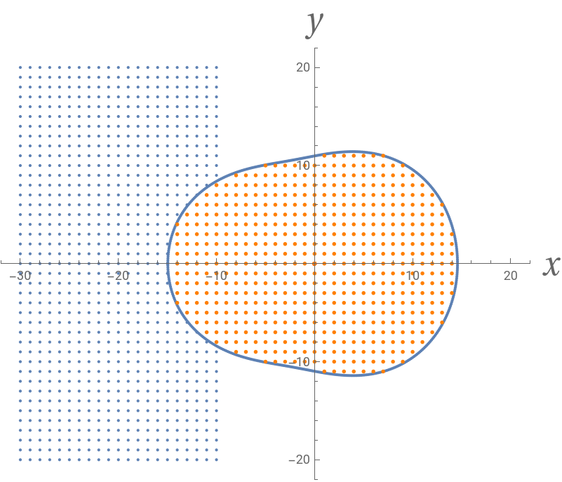
Setting the parameters of the design region where point-like scatterers constructing the acoustic lens are distributed on a square lattice.
Half the length of the design region in the y direction
In[]:=
nm=20;
Half the length of the design region in the x direction
In[]:=
nl=10;
The x - coordinate of the center of the design region
In[]:=
mm=nm;
Number of optimization iterations of the entire system
In[]:=
loop=20;
The list of coordinates of focal points
In[]:=
fp={{0,0}};
The wavenumber of an incident plane wave scaled by the lattice constant d
In[]:=
kd=4Pi;
The effective scattering radius a for a scatterer
In[]:=
a=0.05;
The sound velocities inside and outside the skull , inside the scatterer c and inside the cranial bone are defined here .
c
0
c
1
In[]:=
c0=1480;c=340;c1=4080;
The radius as a function of the angle, which gives a best fit to the cross section of the CT image of a skull built in Mathematica
In[]:=
skul[x_]:=13.142524901619794`+1.9107002874430452`Cos[1.8575980464147388`x]-0.47723727068044897`Cos[3.4370142572581996`x]
The skull is modeled with scatterers of radius a spaced at equal angular intervals.
The angular spacing of the scatterers representing the skull
The angular spacing of the scatterers representing the skull
In[]:=
rsk=Sqrt[2]/2nm+1;nr=Round[rsk];tsk=2ArcSin[a/rsk];
Number of the scatterers representing the skull
In[]:=
nsk=Round[Pi/tsk];
The coordinates of the scatterers representing the skull
In[]:=
Rs=Table[skul[2ntsk-Pi]{Cos[2ntsk-Pi],Sin[2ntsk-Pi]},{n,1,nsk}];
The adaptive ultrasonic lens is modeled as an array of point-like scatterers.
The coordinates of the square-lattice points where the scatterers representing the lens are placed
The coordinates of the square-lattice points where the scatterers representing the lens are placed
In[]:=
Rl=Delete[Union[Flatten[Table[If[i^2+j^2>skul[Im[Log[i+Ij]]]^2,{i,j}],{i,-mm-nl,-mm+nl},{j,-nm,nm}],1]],1];
In[]:=
R=Flatten[{Rl,Rs},1];
We set a square lattice within the target (intracranial) region where an objective function is defined for optimization .
The coordinates of the square-lattice points within the target region
The coordinates of the square-lattice points within the target region
In[]:=
hlp=Flatten[Table[If[i^2+j^2<skul[Im[Log[i+Ij]]]^2,{i,j},{0,0}],{i,-nr,nr},{j,-nr,nr}],1];
Illustration of the design region partially surrounding the skull and of lattice points used to evaluate objective function for optimization.
In[]:=
ListPlotR,AspectRatioAutomatic,PlotRange{{-32,22},{-22,22}},AxesLabelText[Style["x",FontSize24]],TextStyle"y",FontSize24;ListPlot[hlp,AspectRatioAutomatic,PlotStyle{{Orange,Large}}];Show[%%,%]
Out[]=
In[]:=
lfpmn=(Min[Transpose[fp]-(-mm){1,1}])^2;
The Green function in 2D
In[]:=
g[r1_,r2_,k_]:=I/4(BesselJ[0,kSqrt[(r1-r2).(r1-r2)]]+IBesselY[0,kSqrt[(r1-r2).(r1-r2)]])
Setting the scattering ability of a point-like scatterer (an air bubble) representing the lens.
In[]:=
vmax=(1-(c0/c)^2)Pi(kda)^2;
Definition of the scattering potential without the point-like scatterers representing lens
In[]:=
v=Table[0,{l,1,Length[Rl]}];
Initial setting of the scattering potential of the point - like scatterers representing the skull
In[]:=
vs=(1-(c0/c1)^2)Pi(kda)^2Table[1,{l,1,Length[Rs]}];
In[]:=
va=Flatten[{v,vs},1];
Definition of the unknown wave functions at the lattice points where the scatterers representing the lens are placed and the points of the scatterers representing the skull
In[]:=
val=Array[ψ,{Length[R]}];
Setting the inhomogeneous term in the governing equation due to the incident wave.
In[]:=
b=Table[Exp[Ikd{1,0}.R[[i]]],{i,1,Length[R]}];
In[]:=
(*Definingthecoefficientmatrixofthegoverningequationwithoutlens*)mata=Table[If[ij,1+va[[i]]/(4Pi)(2Log[kda/2]+2EulerGamma-1-IPi),-va[[i]]g[R[[i]],R[[j]],kd]],{i,1,Length[R]},{j,1,Length[R]}];(*Settingthegoverningequation*)veca=mata.val;eq=Table[veca[[i]]b[[i]],{i,1,Length[R]}];(*Solvingthegoverningequation*)sol=Solve[eq,val];(*Definingthewavefunctionofthesolution*)phi[r_]:=Exp[Ikd{1,0}.r]+Sum[va[[i]]g[r,R[[i]],kd]ψ[i],{i,1,Length[val]}]/.sol[[1]];(*Computingoneobjectivefunctiondefinedsuchthattheintensityofthesoundfieldvanishesexceptatthefocalpoint(s).*)hf=Sum[If[i^2+j^2<skul[Im[Log[i+Ij]]]^2,Abs[phi[{i,j}]]^2,0],{i,-nr,nr},{j,-nr,nr}];Do[Do[hf=hf-Sum[Abs[phi[fp[[k]]+{i,j}]]^2,{k,1,Length[fp]}],{i,-1,1}],{j,-1,1}];(*Computingandaddingtheotherobjectivefunctionthatisdefinedsothatthesoundfieldintensityisconvexatthefocalpoint(s).*)(*(nm+1)^2/4/lfpmnisaweightingparameter.*)hf=hf+(nm+1)^2/4Sum[(fp[[k,1]]-(-mm))^2/lfpmn(Abs[phi[fp[[k]]+{1,0}]]^2+Abs[phi[fp[[k]]+{0,1}]]^2+Abs[phi[fp[[k]]+{-1,0}]]^2+Abs[phi[fp[[k]]+{0,-1}]]^2-4Abs[phi[fp[[k]]]]^2),{k,1,Length[fp]}];
In[]:=
Adding the initial value of the combined objective function to the list .
In[]:=
ohf=hf;thf={{0,ohf}};
Repeating ``loop'' times to optimize the arrangement of point-like scatterers representing the lens.
In[]:=
Do[(*Repeatingforthenumberofthelatticepointsinthedesignregion.*)Do[(*Chosingonelatticepointwithinthedesignregionusingrandomnumberstotryswitchingwhetherornottoplaceascattererthere.*)l=RandomInteger[{1,Length[Rl]}];(*Storingthevalueofthescatteringpotentialattheselectedpoint.*)ova=va[[l]];(*Switchingwhetherornottoplaceascattererattheselectedpoint.*)If[va[[l]]0,va[[l]]=vmax,va[[l]]=0];(*Solvingthegoverningequationswithscatteringpotentialforthenewarrangementofscatterers.*)mata=Table[If[ij,1+va[[i]]/(4Pi)(2Log[kda/2]+2EulerGamma-1-IPi),-va[[i]]g[R[[i]],R[[j]],kd]],{i,1,Length[R]},{j,1,Length[R]}];veca=mata.val;eq=Table[veca[[i]]b[[i]],{i,1,Length[R]}];sol=Solve[eq,val];(*Definingthewavefunctionforthenewarrangementofscatterers.*)phi[r_]:=Exp[Ikd{1,0}.r]+Sum[va[[i]]g[r,R[[i]],kd]ψ[i],{i,1,Length[val]}]/.sol[[1]];(*Computingthecombinedobjectivefunctionforthenewarrangementofscatterers.*)hf=Sum[If[i^2+j^2<skul[Im[Log[i+Ij]]]^2,Abs[phi[{i,j}]]^2,0],{i,-nr,nr},{j,-nr,nr}];Do[Do[hf=hf-Sum[Abs[phi[fp[[k]]+{i,j}]]^2,{k,1,Length[fp]}],{i,-1,1}],{j,-1,1}];hf=hf+(nm+1)^2/4Sum[(fp[[k,1]]-(-mm))^2/lfpmn(Abs[phi[fp[[k]]+{1,0}]]^2+Abs[phi[fp[[k]]+{0,1}]]^2+Abs[phi[fp[[k]]+{-1,0}]]^2+Abs[phi[fp[[k]]+{0,-1}]]^2-4Abs[phi[fp[[k]]]]^2),{k,1,Length[fp]}];(*TheoptimizationofthenumberandarrangementofscatterersisrealizedbymeansoftheMonteCarlomethodwiththeheatbathmethod.Inordertoavoidthedifficultytonormalizethevalueoftheobjectivefunction,andtomakecomputationfast,however,weemploytheheatbathofzerotemperaturehere,namely,ifthechangeinthevalueoftheobjectivefunctionisnegative,thenewconfigurationisadopted;ifthechangeispositive,theoriginalconfigurationisretained.*)If[hf<ohf,ohf=hf,va[[l]]=ova],{li,1,Length[R]}];(*Addingthenumberofoptimizationandthevalueofthecombinedobjectivefunctionatthetimetothelist.*)thf=AppendTo[thf,{lp,ohf}],{lp,1,loop}]
Dependence of the objective function on the number of optimization iterations of the entire system .
Final arrangement of scatterers within the design region.
Solving the problem for the final arrangement of point-like scatterers and defining the wavefunction of the solution.
Contour plot of sound field intensity within the target region for a final arrangement of scatterers within the design (intracranial) region partially surrounding the skull.
Density plot of sound field intensity within the target region for a final arrangement of scatterers within the design (intracranial) region partially surrounding the skull.
3D plot of sound field intensity within the target region for a final arrangement of scatterers within the design (intracranial) region partially surrounding the skull.
Sound field intensity along the y axis for final arrangement of point - like scatterers within the design region . The background color indicates the outside of the skull.
Sound field intensity along the x axis for final arrangement of scatterers within the design region. The background color indicates the outside of the skull.
CITE THIS NOTEBOOK
CITE THIS NOTEBOOK
Improving the longitudinal spot width of an optimizingly designed point-like scatterer-arrayed transcranial ultrasonic lens
by Ueta Tsuyoshi
Wolfram Community, STAFF PICKS, March 11, 2024
https://community.wolfram.com/groups/-/m/t/3139057
by Ueta Tsuyoshi
Wolfram Community, STAFF PICKS, March 11, 2024
https://community.wolfram.com/groups/-/m/t/3139057