VLE modeling of Ethanol-Water Mixture via Particle Swarm Optimization
Housam Binous
VLE modeling of Ethanol-Water Mixture via Particle Swarm Optimization
Housam Binous
Housam Binous
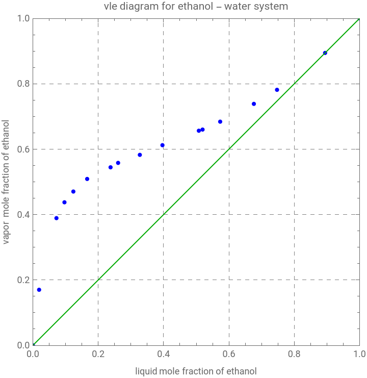
This notebook presents a vapor–liquid equilibrium (VLE) modeling study of the ethanol–water binary system at 1 atm, using experimental x–y–T data spanning the full composition range from pure water to pure ethanol, including the system’s well-known azeotropic behavior. The experimental liquid- and vapor-phase mole fractions of ethanol were extracted and plotted against one another, producing the classic VLE curve that bows above the diagonal (y = x line), reflecting ethanol’s positive deviation from Raoult’s law and its tendency to concentrate in the vapor phase at low-to-moderate liquid compositions.
To model this behavior, the author adopted a two-parameter empirical correlation relating the vapor mole fraction (y) to the liquid mole fraction (x) of ethanol, governed by two adjustable coefficients, a and b (for details see Ref. 1). Rather than fitting these parameters using conventional nonlinear regression (based on NonlinearModelFit), a fitness function was defined as the sum of squared residuals between the experimental and model-predicted vapor mole fractions across all data points, and this objective function was minimized using the Particle Swarm Optimization (PSO) algorithm.
The PSO implementation used a swarm of 50 particles exploring a two-dimensional parameter space (bounded between -20 and 20) over 100 iterations, with an inertia weight of 0.72984 and cognitive/social acceleration coefficients of 1.42, consistent with standard PSO tuning heuristics. The swarm converged rapidly, with the loss dropping from approximately 4.5 × 10⁻³ at iteration 10 to a stable minimum of about 3.21 × 10⁻³ by iteration 50, ultimately locating optimal parameters of a ≈ 10.0825 and b ≈ -1.05271.
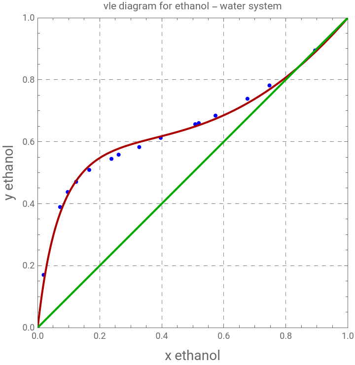
Finally, the PSO-optimized correlation was benchmarked against previously published parameter values (a ≈ 10.065, b ≈ -1.056) obtained via an earlier curve-fitting (see Ref. 2). The PSO-derived fit achieved a marginally lower fitness value (0.00321006 versus 0.00321944), indicating a very slightly improved correlation despite the two parameter sets being numerically close to one another. The resulting model curve was overlaid on the experimental VLE diagram, showing excellent agreement with the data across the full composition range and correctly capturing the pinch point where the equilibrium curve approaches the diagonal near x = y = 1, consistent with the ethanol-rich azeotropic region of the system.
Reference:
[1] M.F.Doherty and M.F.Malone, Conceptual Design of Distillation Systems, Boston : McGraw - Hill, 2001.
[2] https://community.wolfram.com/groups/-/m/t/3117579
In[]:=
(*Ethanol-WaterVLEDataat1atm*)(*Columns:X_EtOH(liquid),Y_EtOH(vapor),T(°C)*)vleData={{0.0,0.0,100.0},{0.019,0.17,95.5},{0.0721,0.3891,89.0},{0.0966,0.4375,86.7},{0.1238,0.4704,85.3},{0.1661,0.5089,84.1},{0.2377,0.5445,82.7},{0.2608,0.558,82.3},{0.3273,0.5826,81.5},{0.3965,0.6122,80.7},{0.5079,0.6564,79.8},{0.5193,0.6599,79.7},{0.5732,0.6841,79.3},{0.6763,0.7385,78.74},{0.7472,0.7815,78.41},{0.8943,0.8943,78.15},{1.0,1.0,78.3}};(*Extractcolumns*)xEtOH=vleData[[All,1]];yEtOH=vleData[[All,2]];tempC=vleData[[All,3]];
In[]:=
(*PlotPsatvsT*)plt1=ListPlot[Transpose@{xEtOH,yEtOH},PlotStyle->{Blue,Thick},Frame->True,FrameLabel->{"liquid mole fraction of ethanol","vapor mole fraction of ethanol"},PlotLabel->"vle diagram for ethanol - water system",GridLines->Automatic,GridLinesStyle->Directive[Gray,Dashed],AspectRatio->1,PlotRange->{{0,1},{0,1}},Epilog->{Darker@Green,Line[{{0,0},{1,1}}]}]
Out[]=
In[]:=
SwarmDim=2;(*3Dproblem*)(*upperandlowerboundsfothesearchdomain*)FitnessLB=-20;FitnessUB=20;c1=1.42;c2=1.42;w=0.72984;(*psoparameters*)Fitness[{a_,b_}]:=Sum[(yEtOH[[i]]-axEtOH[[i]]/(1+(a-1)xEtOH[[i]])-bxEtOH[[i]](1-xEtOH[[i]]))^2,{i,1,Length@tempC}]
In[]:=
Clear[a,b]
In[]:=
(*PSOOptimizer*)psoOptimize[lossFunc_,dim_,lb_,ub_,nParticles_:500,nIter_:50,w_:0.72984,c1_:2,c2_:2]:=Module[{particles,velocities,pbest,pbestScore,gbest,gbestScore,convergence={},r1,r2,score,gbestIdx},(*Initializeparticlesuniformlywithin[lb,ub]ineachdimension*)particles=RandomReal[{lb,ub},{nParticles,dim}];velocities=ConstantArray[0.,{nParticles,dim}];pbest=particles;pbestScore=Table[lossFunc[particles[[i]]],{i,nParticles}];gbestIdx=First@Ordering[pbestScore,1];gbestScore=pbestScore[[gbestIdx]];gbest=pbest[[gbestIdx]];Do[Do[r1=RandomReal[1,dim];r2=RandomReal[1,dim];velocities[[i]]=w*velocities[[i]]+c1*r1*(pbest[[i]]-particles[[i]])+c2*r2*(gbest-particles[[i]]);particles[[i]]+=velocities[[i]];(*keepparticleswithinbounds*)particles[[i]]=Clip[particles[[i]],{lb,ub}];score=lossFunc[particles[[i]]];If[score<pbestScore[[i]],pbest[[i]]=particles[[i]];pbestScore[[i]]=score;];,{i,nParticles}];gbestIdx=First@Ordering[pbestScore,1];gbestScore=pbestScore[[gbestIdx]];gbest=pbest[[gbestIdx]];AppendTo[convergence,gbestScore];If[Mod[t,10]==0,Print["PSO Iter ",t," Loss = ",gbestScore]];,{t,nIter}];{gbest,gbestScore,convergence}];(*RunPSO*){bestPos,bestScore,convergence}=psoOptimize[Fitness,SwarmDim,FitnessLB,FitnessUB,50,100,w,c1,c2];Print["Best position: ",bestPos];Print["Best fitness: ",bestScore];
PSO Iter 10 Loss = 0.00452793
PSO Iter 20 Loss = 0.00339589
PSO Iter 30 Loss = 0.00321189
PSO Iter 40 Loss = 0.00321129
PSO Iter 50 Loss = 0.00321029
PSO Iter 60 Loss = 0.00321007
PSO Iter 70 Loss = 0.00321007
PSO Iter 80 Loss = 0.00321006
PSO Iter 90 Loss = 0.00321006
PSO Iter 100 Loss = 0.00321006
Best position: {10.0825,-1.05271}
Best fitness: 0.00321006
(*Bestposition={10.0825,-1.05271}
In[]:=
a=10.0652;b=-1.05591;(*binaryinteractionparametersfrompreviouscurvefit:https://community.wolfram.com/groups/-/m/t/3117579*)Fitness[{a,b}]
Out[]=
0.00321944
In[]:=
apso=10.0825;bpso=-1.05271;
In[]:=
Show[plt1,Plot[apsox/(1+(apso-1)x)+bpsox(1-x),{x,0,1},PlotStyle->{Thick,Darker@Red}],Frame->True,FrameLabel->{Style["x ethanol",14],Style["y ethanol",14]},GridLines->Automatic,AspectRatio->1,Epilog->{Darker@Green,Thick,Line[{{0,0},{1,1}}]}]
Out[]=