Article abstract
Article abstract
A species distributed across diverse environments may adapt to local conditions. We ask how quickly such a species changes its range in response to changed conditions. Szép et al. (Szép E, Sachdeva H, Barton NH. 2021 Polygenic local adaptation in metapopulations: a stochastic eco-evolutionary model. Evolution75, 1030–1045 (doi:10.1111/evo.14210)) used the infinite island model to find the stationary distribution of allele frequencies and deme sizes. We extend this to find how a metapopulation responds to changes in carrying capacity, selection strength, or migration rate when deme sizes are fixed. We further develop a ‘fixed-state’ approximation. Under this approximation, polymorphism is only possible for a narrow range of habitat proportions when selection is weak compared to drift, but for a much wider range otherwise. When rates of selection or migration relative to drift change in a single deme of the metapopulation, the population takes a time of order to reach the new equilibrium. However, even with many loci, there can be substantial fluctuations in net adaptation, because at each locus, alleles randomly get lost or fixed. Thus, in a finite metapopulation, variation may gradually be lost by chance, even if it would persist in an infinite metapopulation. When conditions change across the whole metapopulation, there can be rapid change, which is predicted well by the fixed-state approximation. This work helps towards an understanding of how metapopulations extend their range across diverse environments.
This article is part of the theme issue ‘Species’ ranges in the face of changing environments (Part II)’.
-1
m
This article is part of the theme issue ‘Species’ ranges in the face of changing environments (Part II)’.
Fixed state and diffusion approximations
Fixed state and diffusion approximations
Derivation of equilibrium under the fixed state approximation
Derivation of equilibrium under the fixed state approximation
In the limit of rare migration, we have fixation of mutations at rate , and in the reverse direction . Note that the number of migrants entering the population is fixed at , independent of the deme size, . We can track the proportion of demes fixed for allele P through time (or the probability that any one deme is fixed):
2sNm
p
1-
-2Ks
2sNm
q
1-
-2Ks
-2Ns
Nm
K
∂
t
2sNm
1-
-2Ks
p
q
-2Ks
P
eq
_
p
p
q
-2Ks
(
1
)If a fraction ρ of demes favour the allele by , and 1-ρ disfavour it, we have that =ρ+(1-ρ), so that at equilibrium:
s
1
p
P
1
P
2
p
ρ(-1)-(-1)
2K(+)
s
1
s
2
2K
s
2
(-1)(-1)
2K
s
1
2K
s
2
2K
s
2
2K(+)
s
1
s
2
(-1)
2K
s
2
2K(+)
s
1
s
2
2K
s
1
(
2
)For =:
s
1
s
2
p
ρ(+1)-1
2Ks
(-1)
2Ks
1
2Ks
2Ks
2Ks
(
3
)The dynamics are:
∂
t
P
1
2Nm
s
1
1-
-2K
s
1
p
Q
1
q
-K
s
1
P
1
∂
t
P
2
2Nm
s
2
1-
-2K
s
2
q
P
2
p
-K
s
2
Q
2
p
P
1
P
2
(
4
)For =:
s
1
s
2
∂
t
P
1
2s Nm
1-
-2Ks
P
1
P
2
Q
1
P
1
-2Ks
-2Ks
P
1
∂
t
P
2
2 Nm
s
1-
-2K
s
P
1
P
2
P
2
Q
2
-2Ks
P
2
(
5
)Example: Ks1=1,Ks2=2
Example:
K=1,K=2
s
1
s
2
WIth these parameters, =1,=2, there is a polymorphism if . The ODE moves to the predicted equilibria when ρ=0.3
Ks
1
Ks
2
0.119<ρ<0.881
tm=1000;{{P1[tm],P2[tm]}/.softP[0.3,{1,2},{0.1,0.3},tm],softPeq[0.3,{1,2.}]}
{{{0.643075,0.00444614}},{0.643075,0.00444614}}
As a check, at the critical ρ, the equilibria tend to fixation:
{{P1[tm],P2[tm]}/.softP[0.133187,{1,2},{0.1,0.3},tm],softPeq[0.133187,{1,2.}],softPeq[0.984124,{1,2.}],softPcrit[{1,2.}]}
{{{0.00365667,9.07071×}},{2.88461×,7.15025×},{1.,1.00002},{0.133187,0.984124}}
-6
10
-6
10
-9
10
This shows the timecourse, on linear and log scales. The blue & black lines give the frequency of the P allele in the rare and the common habitat, and the red line the overall mean. There is a rapid shift in probabilities, almost eliminating the allele from the common habitat (black), and then a slower increase within the rare habitat. These different timescale reflect the different selection strengths.
tm=50;ρρ=0.2;ss=softP[ρρ,{1,2},{0.1,0.3},tm];GraphicsRow[(#[{P1[t]/.ss,P2[t]/.ss,ρρP1[t]+(1-ρρ)P2[t]/.ss},{t,0.01,tm},PlotStyle{Blue,Black,Red}])&/@{Plot,LogLogPlot}]{{P1[tm],P2[tm]}/.ss,{{1,0},{0,1},{ρρ,1-ρρ}}.softPeq[ρρ,{1,2.}]}
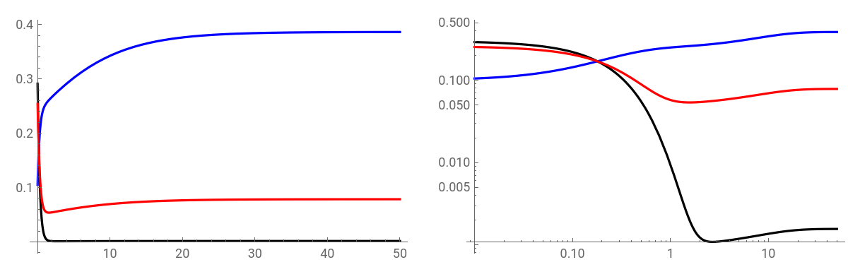
{{{0.386259,0.00155777}},{0.386354,0.0015582,0.0785174}}
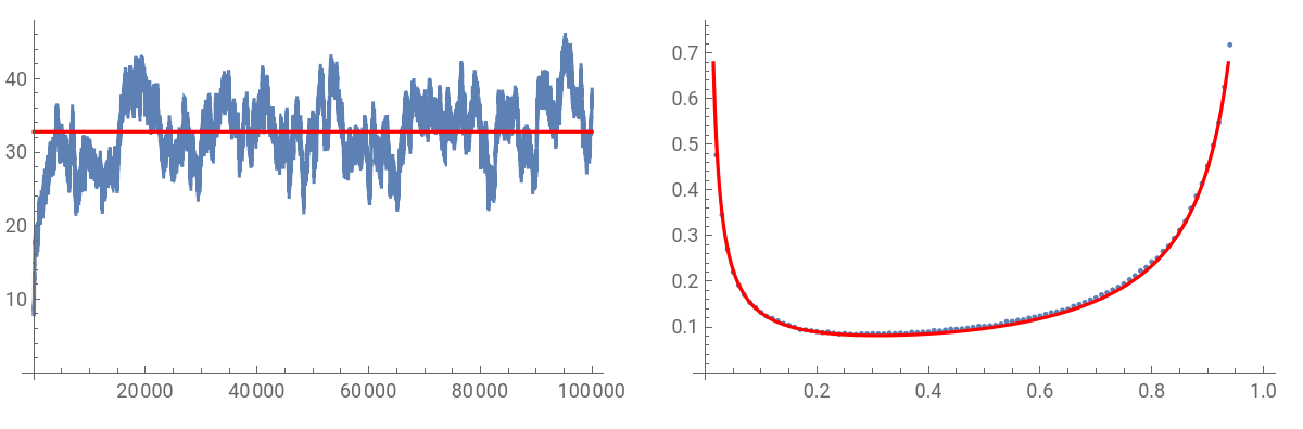
This simulates the version tracking allele frequencies.
K=100;Nm=0.1;s=0.01;L=100;pb=0.079;p=ConstantArray[pb,L];T=;Timing[nnp=runP[K,Nm,p,s,T];]
5
10
{231.595,Null}
The frequency in the rare habitat fluctuates around the predicted mean, and is close to the diffusion.
bc=BinCounts[Flatten[nnp〚;;-1〛],{0,101}];GraphicsRowShow[ListLinePlot[Transpose[{Range[0,T,10],Mean/@nnp〚1;;-1;;10〛}]],Plot[KmP[Nm,pb,Ks],{t,0,T},PlotStyleRed]],ShowListPlotTransposeRange0,1,,,Plot[ψP[p,Nm,pb,Ks],{p,0,1},PlotStyleRed]
4
10
1
K
bc
T-
4
10
Derivation of equilibrium under the diffusion approximation
Derivation of equilibrium under the diffusion approximation
Now, consider the full version, where allele frequencies are distributed according to the diffusion, There is an explicit formula for , given :
[p]
p
[p]=(2Nm+1;2Nm+1;2Ks)(2Nm;2Nm;2Ks)
p
1
F
1
p
1
F
1
p
(
6
)If selection is equal and opposite, we can solve for :
p
p
p
1
F
1
p
1
F
1
p
1
F
1
p
1
F
1
p
(
7
)By setting =0or1, one can find the range of ρ for which polymorphism is possible. The hypergeometrics simplify to:
p
1-g[-]
Ks
2
g[]-g[-]
Ks
1
Ks
2
g[]-1
Ks
2
g[]-g[-]
Ks
2
Ks
1
1
F
1
p
1
F
1
p
-2Nm
(2)
Ks
2
2
Ks
2
Ks
2
(
8
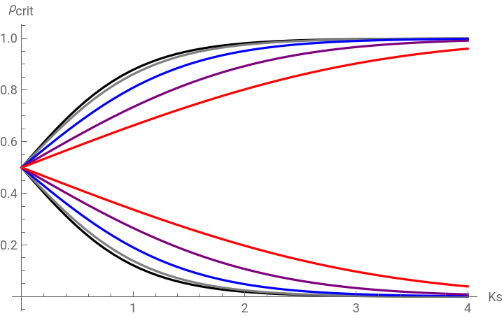
)This shows the critical ρ as a function of (assuming symmetric selection ±s in the two habitats).
Ks
Nm=0.01,0.1,0.4,1,2(black…red)
gr1[Nm_,c_]:=Plot[ρCrit[Nm,{Ks,Ks}],{Ks,0,4},AxesLabel{"Ks",""},PlotStylec];Show[MapThread[gr1,{{0.01,0.1,0.4,1,2},{Black,Gray,Blue,Purple,Red}}]]
ρ
crit
Szep et al. give . This compares the prediction (black) with Ks (red). It seems to be accurate only for Ks<2:
K=log+Nm(1-2ρ)
s
crit
1
2
1-ρ
ρ
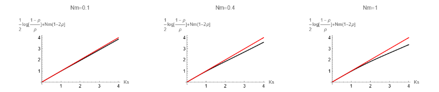
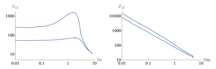
Fig. 4 - response time for a single deme
Fig. 4 - response time for a single deme
This is derived using the transition matrix for a single deme. The codes that generated the figure are in the closed cells below (to open them, click on cell cell properties open).
Derivation of the transition matrix
Derivation of the transition matrix
To try this approach numerically, we must include a low rate of mutation, so that there is a stationary state. One would also like to find he dynamics of the distribution of states, which can be done most simply by iterating a discrete-time version.
One could imagine (for a large # of loci) a diffusion approximation to this transition matrix.
Accuracy of the fixed-state approximation
Accuracy of the fixed-state approximation
Simulations
Simulations
The top row shows the mean allele frequencies at 10 loci, and the overall mean (red), in the two habitats (left, right). The magenta curve shows the fixed state approximation, which underestimates the migration load. The bottom row is similar, but shows the fraction of demes >50% instead of the mean allele frequency - which is closer to the spirit of the fixed state approximation. There is still a substantial discrepancy, though perhaps it is slightly smaller.
The top row shows the individual allele frequency trajectories at 10 loci in one (arbitrarily chosen) deme, to get a sense of whether the fixed-state approximation is appropriate. The trajectories do more or less make jumps between low & high frequency. The bottom row shows the mean across all demes, which declines from the initial ρ=0.2, as the adaptive allele is lost from some fraction of demes in the rarer habitat.
The top row shows the mean allele frequencies at 10 loci, and the overall mean (red), in the two habitats (left, right). The magenta curve shows the fixed state approximation, which underestimates the migration load. The bottom row is similar, but shows the fraction of demes >50% instead of the mean allele frequency - which is closer to the spirit of the fixed state approximation. There is still a substantial discrepancy, though perhaps it is slightly smaller.
The top row shows the mean allele frequencies at 40 loci, and the overall mean (red), in the two habitats (left, right). The magenta curve shows the fixed state approximation, which underestimates the migration load. The bottom row is similar, but shows the fraction of demes >50% instead of the mean allele frequency - which is closer to the spirit of the fixed state approximation.
There is still a substantial discrepancy,with both means of measurement. Agreement is good for the common habitat, where the introgressing allele is rare (0.0024), but poor for the rare habitat, where it is at 0..256, compared with a prediction of 0.397
The top row shows the individual allele frequency trajectories at 10 of the 40 loci in one (arbitrarily chosen) deme, to get a sense of whether the fixed-state approximation is appropriate. The trajectories do more or less make jumps between low & high frequency. The bottom row shows the mean across all demes, which declines from the initial ρ=0.2, as the adaptive allele is lost from some fraction of demes in the rarer habitat. However, there is considerable variation across loci, because of the concerted evolution across demes. In the infinite-deme limit, there would be no such variability.
The overall mean in the metapopulation changes smoothly, but converges to a substantially lower value than expected. The 10 individual loci follow markedly different paths, which may account for this variability:
The observed and predicted mean frequencies are close, and approaching the equilibrium, for the common habitat, but not the rare one:
Fixed-state recursion with 10, 40 demes:
Fixed-state recursion with 10, 40 demes:
Setting up the transition matrix
Setting up the transition matrix
There are 2151 rates in a 451×451 matrix, :
Change through time
Change through time
Regardless of the starting point, the distribution converges to the stationary distribution:
This sets up the transition matrix approximation.
Figure xx. Mean allele frequency through time, in the 20 demes where the focal allele is favoured (top), and the 80 demes where it is not (bottom). Thin lines show allele frequencies at 40 loci, averaged over demes; the red line shows the overall mean. The black curve shows the fixed state approximation.
The top row shows the individual allele frequency trajectories at 10 of the 40 loci in one (arbitrarily chosen) deme, to get a sense of whether the fixed-state approximation is appropriate. The trajectories do more or less make jumps between low & high frequency. The bottom row shows the mean across all demes, which declines from the initial ρ=0.2, as the adaptive allele is lost from some fraction of demes in the rarer habitat. However, there is considerable variation across loci, because of the concerted evolution across demes. In the infinite-deme limit, there would be no such variability.
The overall mean in the metapopulation changes smoothly, but converges to a substantially lower value than expected. The 10 individual loci follow markedly different paths, which may account for this variability:
The observed and predicted mean frequencies are close, and approaching the equilibrium, for the common habitat, but not the rare one:
Definitions
Definitions