We use symbolic capabilities of Mathematica in order to solve Example 18.6 - 3 of Ref . 1, which is reproduced below.
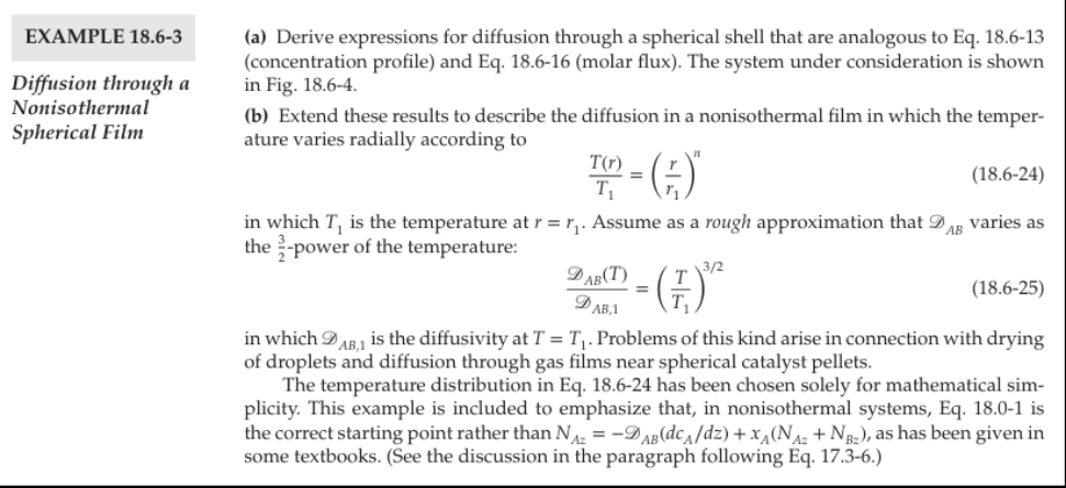
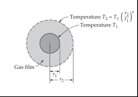
Part (a) case when n=0 or isothermal problem
Part (a) case when n=0 or isothermal problem
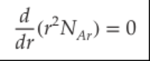
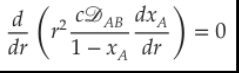
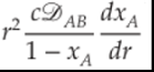
let us find xA(r) as a function of A
In[]:=
sol=First@DSolve[{r^2c/(1-xA[r])D[xA[r],r]==A,xA[r1]==xA1,xA'[r1]==A/(r1^2c)(1-xA1)},{xA[r]},r]//FullSimplify
AB
AB
Out[]=
xA[r]1+(-1+xA1)
A(-r+r1)
crr1
AB
now let us find log[(1-xA(r))/(1-xA1)] as a function of A
In[]:=
Log[(1-xA[r]/.sol)/(1-xA1)]//FullSimplify
Out[]=
Log
A(-r+r1)
crr1
AB
we use the boundary condition xA(r=r2)=xA2 in order to determine A
In[]:=
sol1=First@Solve==Log[(1-xA2)/(1-xA1)],A
A(-r2+r1)
cr2r1
AB
Out[]=
A
cr1r2Log
1-xA2
1-xA1
AB
r1-r2
final form of log[(1-xA(r))/(1-xA1)] is found below
In[]:=
(1-xA[r])/(1-xA1)/.sol/.sol1//FullSimplify
Out[]=
(-r+r1)r2
r(r1-r2)
-1+xA2
-1+xA1
finally let us check that our result is equivalent to the solution given in Ref . 1 :
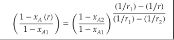
In[]:=
(-r+r1)r2
r(r1-r2)
-1+xA2
-1+xA1
((1/r1-1/r)/(1/r1-1/r2))
-1+xA2
-1+xA1
Out[]=
0
Molar flow rate determination
In[]:=
WA=-A4π/.sol1
Out[]=
-
4cπr1r2Log
1-xA2
1-xA1
AB
r1-r2
Part (b) nonisothermal case
Part (b) nonisothermal case
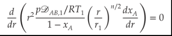
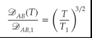
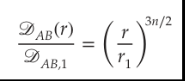
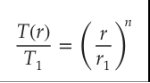
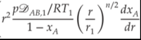
let us find xA(r) as a function of A
Without loss of generality let us assume n = 3
In[]:=
n=3;
In[]:=
sol=First@DSolve[{r^2p/R/T1/(1-xA[r])(r/r1)^(n/2)D[xA[r],r]==A,xA[r1]==xA1,xA'[r1]==A/(r1^2p)RT1(1-xA1)},{xA[r]},r]//FullSimplify
AB1
AB1
Out[]=
xA[r]1+(-1+xA1)
-
2AR-T1
3
r
r
r1
3
r1
5pr1
3
r
AB1
now let us find log[(1-xA(r))/(1-xA1)] as a function of A
In[]:=
Log[(1-xA[r]/.sol)/(1-xA1)]//FullSimplify
Out[]=
Log
-
2AR-T1
3
r
r
r1
3
r1
5pr1
3
r
AB1
we use the boundary condition xA(r=r2)=xA2 in order to determine A
In[]:=
sol1=First@Solve-==Log[(1-xA2)/(1-xA1)],A
2AR-T1
3
r2
r2
r1
3
r1
5pr1
3
r2
AB1
Out[]=
A-
5pr1Log
3
r2
1-xA2
1-xA1
AB1
2R-T1
3
r2
3
r1
r2
r1
final form of log[(1-xA(r))/(1-xA1)] is found below
In[]:=
(1-xA[r])/(1-xA1)/.sol/.sol1//FullSimplify
Out[]=
3
r
r
r1
3
r1
3
r2
3
r
3
r2
3
r1
r2
r1
-1+xA2
-1+xA1
Molar flow determination
In[]:=
WA=-A4π/.sol1//Factor
Out[]=
10pπr1Log
3
r2
1-xA2
1-xA1
AB1
R-T1
3
r2
3
r1
r2
r1
finally let us check that our result is equivalent to the solution given in Ref . 1 :

In[]:=
Simplify-4π(p/R/T1)(1+n/2)Log((1/r1)^(1.+n/2)-(1/r2)^(1.+n/2))r1^(n/2.),r1>0&&r2>0
10pπr1Log
3
r2
1-xA2
1-xA1
AB1
R-^(1./2)T1
3
r2
3
r1
r2
r1
AB1
1-xA2
1-xA1
Out[]=
0.
References
References
[1] R. Byron Bird, Warren E. Stewart, Edwin N. Lightfoot, and Daniel Klingenberg, Introductory Transport Phenomena, NY: Wiley, 2015.
CITE THIS NOTEBOOK
CITE THIS NOTEBOOK
Diffusion through a nonisothermal spherical film
by Housam Binous and Ahmed Bellagi
Wolfram Community, STAFF PICKS, September 23, 2025
https://community.wolfram.com/groups/-/m/t/3549676
by Housam Binous and Ahmed Bellagi
Wolfram Community, STAFF PICKS, September 23, 2025
https://community.wolfram.com/groups/-/m/t/3549676