Determining Extrema of the Himmelblau Function via Particle Swarm Optimization
Housam Binous
Determining Extrema of the Himmelblau Function via Particle Swarm Optimization
Housam Binous
Housam Binous
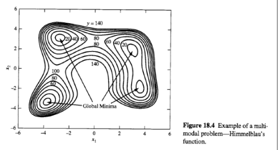
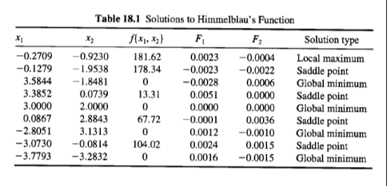
This notebook numerically locates and classifies all stationary points of Himmelblau’s test function defined by:f(x1,x2) = (x1^2+x2-11)^2+(x1+x2^2-7)^2using Particle Swarm Optimization (PSO) launched from many random initial swarms/seeds. The resulting candidate points are collected into a stationarypoints table, then deduplicated (via a Norm[#1-#2] < edgeDedupTol tolerance test) into a final set called allninestationaryPts — confirming there are exactly nine stationary points. Each point is then classified (minimum, maximum, or saddle) by evaluating the Hessian matrix and its eigenvalues at that point (positive definite → minimum, negative definite → maximum, mixed signs → saddle), and the results are tabulated alongside the function value f(x1,x2) at each point.Why exactly 9 stationary points — Bézout’s TheoremSetting the gradient to zero gives two equations:4x1 (x1^2+x2-11) + 2 (x1+x2^2-7)=02 (x1^2+x2-11) + 4 x2 (x1+x2^2-7)=0Each of these is a cubic (degree-3) plane curve in (x1, x_2) — the leading terms 4x1^3 and 4x2^3 confirm the degree. Bézout’s theorem states that two plane algebraic curves of degrees m and n, with no common component, intersect in at most mxn points (counted with multiplicity, over the complex projective plane). Here, m=n=3, so the theorem bounds the number of stationary points at 3x3 = 9. For Himmelblau’s function this bound is achieved exactly, with all 9 intersection points real and finite: 4 local minima (the famous equal-valued global minima, f=0), 4 saddle points, and 1 local maximum — which is precisely what the PSO search and Hessian classification in this notebook recover numerically.Reference:[1] Seider, W. D., Seader, J. D., & Lewin, D. R. (2004). Product and Process Design Principles: Synthesis, Analysis, and Evaluation (2nd ed.). New York: John Wiley & Sons.
In[]:=
(*ParticleSwarmOptimizer*)clipMatrix[mat_,lbv_,ubv_]:=Transpose[MapThread[Clip[#1,{#2,#3}]&,{Transpose[mat],lbv,ubv}]];clampMatrix[mat_,vmaxv_]:=Transpose[MapThread[Clip[#1,{-#2,#2}]&,{Transpose[mat],vmaxv}]];
In[]:=
psoOptimize[lossFunc_,dim_,lb_,ub_,nParticles_:30,nIter_:100,wMax_:0.9,wMin_:0.4,c1_:1.42,c2_:1.42,vClampFrac_:0.2,seed_:1]:=Module[{particles,velocities,pbest,pbestScore,gbest,gbestScore,convergence={},r1,r2,scores,gbestIdx,vmax,wIter},SeedRandom[seed];vmax=vClampFrac*(ub-lb);particles=Transpose@Table[RandomReal[{lb[[i]],ub[[i]]},nParticles],{i,dim}];velocities=ConstantArray[0.,{nParticles,dim}];pbest=particles;pbestScore=lossFunc/@particles;gbestIdx=First@Ordering[pbestScore,1];gbestScore=pbestScore[[gbestIdx]];gbest=pbest[[gbestIdx]];Do[wIter=wMax-(wMax-wMin)*(j-1)/(nIter-1);r1=RandomReal[1,{nParticles,dim}];r2=RandomReal[1,{nParticles,dim}];velocities=wIter*velocities+c1*r1*(pbest-particles)+c2*r2*(ConstantArray[gbest,nParticles]-particles);velocities=clampMatrix[velocities,vmax];particles+=velocities;particles=clipMatrix[particles,lb,ub];scores=lossFunc/@particles;pbest=MapThread[If[#3<#2,#1,#4]&,{particles,pbestScore,scores,pbest}];pbestScore=MapThread[Min,{pbestScore,scores}];gbestIdx=First@Ordering[pbestScore,1];If[pbestScore[[gbestIdx]]<gbestScore,gbestScore=pbestScore[[gbestIdx]];gbest=pbest[[gbestIdx]];];AppendTo[convergence,gbestScore],{j,nIter}];{gbest,gbestScore}];
In[]:=
(*ClassifyeachconvergedpointviatheHessianeigenvalues*)classify[{x_,y_}]:=Module[{eig},eig=Eigenvalues[hessf[x,y]];Which[Max[Abs[eig]]>1*^-4&&Min[eig]>0,"minimum",Max[Abs[eig]]>1*^-4&&Max[eig]<0,"maximum",Min[eig]<0&&Max[eig]>0,"saddle"]];
In[]:=
(*FindingallcriticalpointsviaPSObyminimizing||gradf||^2Himmelblaufunction:f(x1,x2)=(x1^2+x2-11)^2+(x1+x2^2-7)^2*)ClearAll[f,loss,gradf,hessf];(*DefinetheHimmelblaufunction*)f[x1_,x2_]:=(x1^2+x2-11)^2+(x1+x2^2-7)^2
In[]:=
vars={x,y};gradf[x_,y_]:=Evaluate@D[f[x,y],{vars}](*Gradient:{∂f/∂x,∂f/∂y}*)hessf[x_,y_]:=Evaluate@Outer[D[f[x,y],{#1,1},{#2,1}]&,vars,vars](*HessianusingOuter*)
In[]:=
gradf[x,y]
Out[]=
{4x(-11++y)+2(-7+x+),2(-11++y)+4y(-7+x+)}
2
x
2
y
2
x
2
y
In[]:=
hessf[x,y]//MatrixForm
Out[]//MatrixForm=
2+8 2 x 2 x | 4x+4y |
4x+4y | 2+8 2 y 2 y |
In[]:=
(*ObjectivePSOwillminimize:squarednormofthegradient*)loss[{x_,y_}]:=Total[gradf[x,y]^2];
In[]:=
(*Runseveralindependentswarms(differentrandomseeds)sowe'relikelytolandonallcriticalpoints*)results=Table[psoOptimize[loss,2,{-6,-6},{6,6},30,100,0.9,0.4,1.42,1.42,0.2,seed],{seed,1,100}];
In[]:=
Print["Run gbest (x,y) ||grad||^2 classification"];Do[With[{pt=results[[k,1]],val=results[[k,2]]},Print[k," ",NumberForm[pt,{6,4}]," ",ScientificForm[val,3]," ",classify[pt]]],{k,Length[results]}];
Removing duplicates yields only 9 stationary points in agreement with Bezout theorem and Table 18.1 of Ref . 1