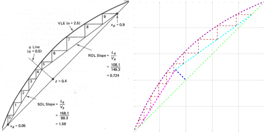
The present calculation is adapted from adapted from example 8-2 textbook by Luyben and Wenzel (Ref. 1).
The notebook computes the number of equilibrium stages for a binary ideal mixture with relative volatility equal to 2.5 . The feed is a two phase mixture with a feed quality is equal to 0.5 . The distillate, feed and bottom mole fractions are 0.9, 0.4 and 0.05, respectively . The minimum reflux ratio and pinch point position are calculated . The reflux ratio is taken equal to 2.625. We draw the McCabe and Thiele Diagram and get the number of theoretical plates equal to 9 plus a partial reboiler. The optimum feed plate position is stage 5 counting from the top.
The notebook computes the number of equilibrium stages for a binary ideal mixture with relative volatility equal to 2.5 . The feed is a two phase mixture with a feed quality is equal to 0.5 . The distillate, feed and bottom mole fractions are 0.9, 0.4 and 0.05, respectively . The minimum reflux ratio and pinch point position are calculated . The reflux ratio is taken equal to 2.625. We draw the McCabe and Thiele Diagram and get the number of theoretical plates equal to 9 plus a partial reboiler. The optimum feed plate position is stage 5 counting from the top.
Equilibrium curve for a constant relative volatility equal to 2.5
In[]:=
equilb=Function[With[{a=2.5},(a#/(1+(a-1)#))]]
Out[]=
With{a=2.5},&
a#1
1+(a-1)#1
In[]:=
plt0=Plot[equilb[x],{x,0,1},PlotStyle{Dashed,Darker@Magenta},FrameLabel->{Style["liquid mole fraction",14],Style["vapor mole fraction",14]},Epilog{Dashed,RGBColor[0,1,0],Line[{{0,0},{1,1}}]},Frame->True,GridLines->Automatic,PlotRange->{{0,1},{0,1}}];
Distillate, Bottom and Feed Compositions
In[]:=
xd=0.9;
In[]:=
xb=0.05;
In[]:=
zf=0.4;
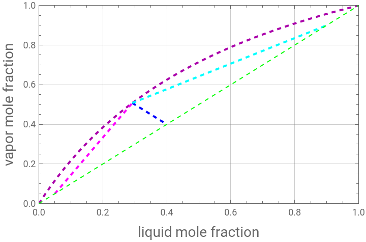
Drawing Feed Line, determining of the pinch point and obtaining the Minimum Reflux Ratio. The feed is a two phase mixture with a feed quality is q=0.5.
In[]:=
feed=Function[With[{q=0.5},(q#/(q-1)-zf/(q-1))]]
Out[]=
With{q=0.5},-&
q#1
q-1
zf
q-1
In[]:=
With{q=0.5`},-&
q#1
q-1
zf
q-1
Out[]=
With{q=0.5},-&
q#1
q-1
zf
q-1
In[]:=
pinch=FindRoot[feed[x]equilb[x],{x,0.5}]
Out[]=
{x0.292159}
In[]:=
xpinch=pinch[[1,2]]
Out[]=
0.292159
In[]:=
ypinch=feed[xpinch]
Out[]=
0.507841
In[]:=
plt1=Plot[feed[x],{x,xpinch,zf},PlotStyle{Dashed,RGBColor[0,0,1]},PlotRange{{0,1},{0,1}},Frame->True,GridLines->Automatic,PlotRange->{{0,1},{0,1}}];
In[]:=
opertRect=Function[ypinch+(#-xpinch)/(xd-xpinch)(xd-ypinch)]
Out[]=
ypinch+&
(#1-xpinch)(xd-ypinch)
xd-xpinch
In[]:=
opertRect[xd]
Out[]=
0.9
In[]:=
opertRect[xpinch]
Out[]=
0.507841
In[]:=
opertStrp=Function[ypinch+(#-xpinch)/(xb-xpinch)(xb-ypinch)]
Out[]=
ypinch+&
(#1-xpinch)(xb-ypinch)
xb-xpinch
In[]:=
opertStrp[xpinch]
Out[]=
0.507841
In[]:=
opertStrp[xb]
Out[]=
0.05
In[]:=
plt2=Plot[opertRect[x],{x,xpinch,xd},PlotStyle{Dashed,RGBColor[0,1,1]},Frame->True,GridLines->Automatic,PlotRange->{{0,1},{0,1}}];
In[]:=
plt3=Plot[opertStrp[x],{x,xb,xpinch},PlotStyle{Dashed,RGBColor[1,0,1]},Frame->True,GridLines->Automatic,PlotRange->{{0,1},{0,1}}];
In[]:=
Show[plt0,plt1,plt2,plt3]
Out[]=
In[]:=
Rmin=(xd-ypinch)/(xd-xpinch)/(1-(xd-ypinch)/(xd-xpinch))//Simplify
Out[]=
1.81822
Reflux ratio is taken equal to 2.625
In[]:=
R=2.625
Out[]=
2.625
Operating line of the rectifying section
In[]:=
OpRect=Function[R/(R+1)#+xd/(R+1)]
Out[]=
R#1
R+1
xd
R+1
Intersection Between Feed Line and Rectifying Operating Line
In[]:=
inters=FindRoot[feed[x]OpRect[x],{x,0.5}]
Out[]=
{x0.32}
In[]:=
xinters=inters[[1,2]]
Out[]=
0.32
In[]:=
yinters=OpRect[xinters]
Out[]=
0.48
Slopes of feed line, stripping and rectifying operating Line
In[]:=
(xb-yinters)/(xb-xinters)
Out[]=
1.59259
In[]:=
q
q-1
Out[]=
-1.
Drawing feed line and operating lines for rectifying and stripping sections
In[]:=
plt4=Plot[OpRect[x],{x,xinters,xd},PlotStyle{Dashed,RGBColor[0,1,1]},Frame->True,GridLines->Automatic,PlotRange->{{0,1},{0,1}}];
In[]:=
OpStrp=Function[yinters+(#-xinters)/(xb-xinters)(xb-yinters)]
Out[]=
yinters+&
(#1-xinters)(xb-yinters)
xb-xinters
In[]:=
plt5=Plot[OpStrp[x],{x,xb,xinters},PlotStyle{Dashed,RGBColor[1,0,1]},Frame->True,GridLines->Automatic,PlotRange->{{0,1},{0,1}}];
In[]:=
plt6=Plot[feed[x],{x,xinters,zf},PlotStyle{Dashed,RGBColor[0,0,1]},PlotRange{{0,1},{0,1}},Frame->True,GridLines->Automatic,PlotRange->{{0,1},{0,1}}];
In[]:=
Show[plt0,plt6,plt4,plt5]
Out[]=
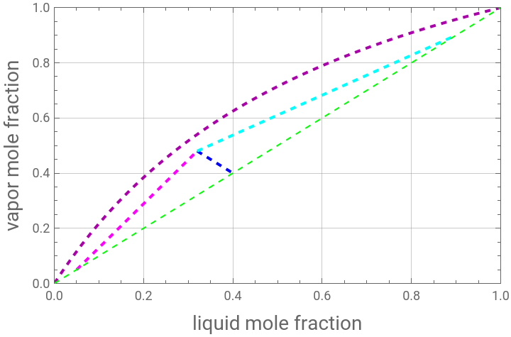
Computing the number of equilibrium stages and Drawing the McCabe and Thiele Diagram. 9 stages and a partial reboiler are need for this distillation problem. Optimum feed stage location is fifth stage counting from the top.
In[]:=
x=.;y=.;
In[]:=
y[0]=xd;x[0]=xd;i=0;
In[]:=
While[x[i]>xinters,{Print[x[i]," ",i," ",y[i]],v=FindRoot[y[i]equilb[u],{u,0.5}][[1,2]],t=OpRect[v],If[v>xinters,{x[i+1]=v,y[i+1]=t}],i++}]
0.9 0 0.9
0.782609 1 0.814993
0.637953 2 0.710242
0.495067 3 0.606773
0.381656 4 0.524648
In[]:=
i=i-1
Out[]=
4
Superposing our graph with its counterpart reported in Ref . 1
References
References
◼
[1] William L. Luyben and Leonard A. Wenzel, Chemical Process Analysis: Mass and Energy Balances, NJ: Prentice-Hall, 1988.
CITE THIS NOTEBOOK
CITE THIS NOTEBOOK
McCabe & Thiele construction
by Housam Binous and Ahmed Bellagi
Wolfram Community, STAFF PICKS, December 23, 2024
https://community.wolfram.com/groups/-/m/t/3342959
by Housam Binous and Ahmed Bellagi
Wolfram Community, STAFF PICKS, December 23, 2024
https://community.wolfram.com/groups/-/m/t/3342959