ABSTRACT (original article): Small changes in the chemical potential at a semiconductor interface can result in dramatic changes to the space-charge layer that underpins applications in the electronic and photovoltaic industries as well as in photoelectrochemical cells for fuel production. There has hence been great interest in techniques that directly probe the space-charge layer, yet many fail at the semiconductor–electrolyte interface due to the potential drop in the electric double-layer region of the electrolyte. This article demonstrates that photovoltages, obtained from straightforward cyclic voltammetry measurements, provide an experimental and quantitative approach for characterizing the semiconductor–electrolyte interface. Key parameters accessible through this approach include the flat-band potential (Efb), the fraction of the total potential that drops across the space-charge layer (γsc) and the electric double layer, as well as the surface recombination lifetime (τs). We report photovoltage measurements for p-type Si(111) photoelectrodes in contact with electrolytes containing redox-active species with a range of known reduction potentials that exceed the 1.1 eV bandgap. In tetrabutylammonium [NBu4]+ electrolyte, the flat-band potential determined for hydrogen-terminated (p-Si–H), methyl-terminated (p-Si–CH3), and chemically oxidized (p-Si–cSiOx) surfaces were −0.02, −0.31, and 0.30 V vs Fc+/0, respectively, agreeing well with expected shifts arising from surface dipole modifications. The quantitative analysis also reveals that 67% of the applied bias drops across the space-charge layer for p-Si–H, 73% for p-Si–CH3, and only 44% for p-Si–cSiOx. The remaining potential drop is attributed to the interfacial surface layer, which consists of a molecular dipole or oxide overlayer, and the Helmholtz layer within the electrolyte. When the larger [NBu4]+ electrolyte was replaced with Li+, the flat-band position showed minimal changes, but the fraction of the potential drop across the space-charge layer increased significantly, consistent with the small cation altering the structure of the electric double layer. CITATION (original article): Pierpaolo Vecchi, Matthew J. Goodwin, Devon P. Leimkuhl, John C. Dickenson, Gabriela P. Bein, Megan N. Jackson, James F. Cahoon, Jillian L. Dempsey, Gerald J. Meyer, and Renato N. Sampaio, Quantitative Analysis of the Semiconductor–Electrolyte Interface Using Cyclic Voltammetry Measurements, Journal of the American Chemical Society 2026 148 (10), 10491-10505. https://doi.org/10.1021/jacs.5c18135
This notebook evaluates the changes in electrostatic potential of a semiconductor using solutions to the Poisson-Boltzmann and carrier transport equations. The underlying formalism follow the mathematical treatment of Many, Goldstein, and Grover,[1] with later extensions by Kronik an co-workers.[2] The resulting model curves are used to fit photovoltage data obtained from cyclic voltammetry of illuminated semiconductors in contact with redox-active analytes.[3] From this analysis key properties of the semiconductor-electrolyte interface can be extracted, including the flat-potential, the fraction of the applied potential that drops across the semiconductor space-charge region, and the surface recombination lifetime. In work published in the Journal of the American Chemical Society, Sampaio and co-authors demonstrate that photovoltage analysis provides a broadly applicable and experimentally accessible approach for probing the the energetics of semiconductor-electrolyte interfaces, with direct implications for the design and optimization of photoelectrons in solar energy conversion and related interfacial electron transfer processes.[3]
Clear Kernel and Import Experimental Data
Clear Kernel and Import Experimental Data
In using external experimental data, then select folder path. Choose file containing only x-y pairs without titles.
In[]:=
ClearAll;Unprotect;Clear["Global`*"]
SetDirectory["FOLDER PATH"];ϕphdata=Import["FILE_NAME.csv"];
Using Internal Reference Data
Using Internal Reference Data
If experimental data is not available, then use this line to create a reference data for modeling and fitting.
In[]:=
ϕphdata={{-0.749,0.04033},{-0.8275,0.085},{-1.159,0.25083},{-1.214,0.326},{-1.247,0.33},{-1.329,0.41933},{-1.658,0.4405},{-1.744,0.43283},{-1.873,0.408},{-1.901,0.41817}};
Universal Constants and Physical Properties of Semiconductor
Universal Constants and Physical Properties of Semiconductor
In this section, enter the values for all necessary universal constants and semiconductor properties.
Universal Constants
kT=0.0259;(*productoftheBoltzmanconstantandtemperature,atroomtemperature(298.15K)inunitsofeV*)q=1.602*10^-19;(*elementarychargeofanelectron,C*)ε0=8.854*10^-12;(*vacuumpermittivity,F/m*)
Optical Properties of Silicon
In[]:=
α=53500;(*absorptioncoefficient,1/mat850nm,photonenergy1.458eV*)R=0.32;(*reflectivity,at850nm*)G[Io_,x_]:=α*(1-R)*Io/(1.458*q)Exp[-α*x];(*generationrate,fora850nmexcitation,inunitsofphotons/m^3.IoisprovidedinunitsofW/m^2,andxistheunidemenisonalaxysalongthesiliconinunitsofmeters*)
Material Properties of Silicon
In[]:=
dwafer=380*10^-6;(*thicknessofthesiliconwafer,inmeters*)dsc=3*10^-6;Na=1.4*10^21;(*dopingdensityofsilicon,1/m^3*)ni=8.3*10^15;(*intrinsiccarrierdensityofsilicon,1/m^3*)p0=Na;(*equilibriumdensityofmajoritycarriers,1/m^3*)n0=ni^2/Na;(*equilibriumdensityofminoritycarreirs,1/m^3*)εr=11.7(*relativepermittivityofsilicon*);
Electron Properties of Silicon
In[]:=
Dn=0.003598;(*diffusioncoefficientofelectronsinsilicon,m^2/s*)μn=1306.8*10^-4;(*mobilityofelectronsinsilicon,m^2/(V.s)*)
Carrier Lifetime and Surface recombination Velocity
In[]:=
τEff[τb_,τs_]:=1/(1/τb+1/τs);(*effectivecarrierlifetime.τbandτsarethebulkandsurfacerecombinationlifetimesrespectivetly,allinunitsofseconds*)S[τs_]:=dwafer/τs;(*surfacerecombinationvelocity,m/s*)
Simulation of the Photogenerated Excess Carrier Distribution
Simulation of the Photogenerated Excess Carrier Distribution
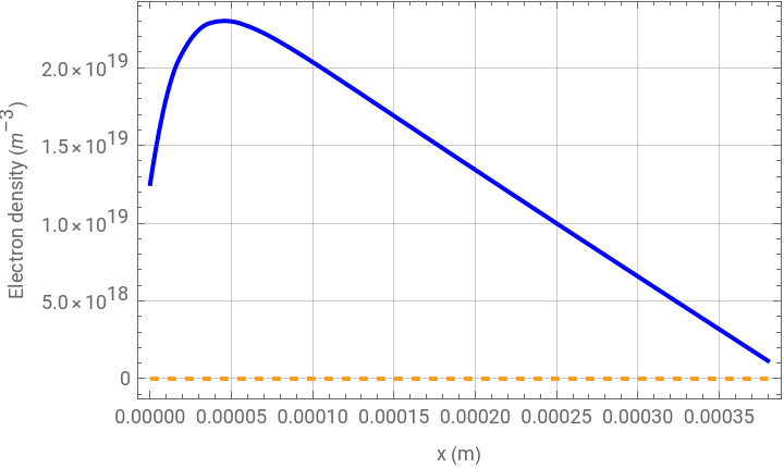
In this section, the differential equation describing generation, recombination and transport of photogenerated excess carriers is solved numerically for given values of Irradiance (Io), bulk recombination lifetime (τb), and surface recombination lifetime (τs).
Numerical Solver to the Continuity Equation
Numerical Solver to the Continuity Equation
Surface recombination are described as boundary fluxes using Neumann boundary conditions to both surfaces of the semiconductor.
In[]:=
diffusionPDE[Io_,τb_,τs_]:=-Dn*D[u[x],{x,2}]-G[Io,x]+u[x]/τEff[τb,τs];ufun[Io_,τb_,τs_]:=NDSolveValue[{diffusionPDE[Io,τb,τs]==NeumannValue[-(dwafer/(Dnτs))*u[x],x==0]+NeumannValue[-(dwafer/(Dnτs))*u[x],x==dwafer]},u,{x,0,dwafer}];electronProfile[Io_,τb_,τs_]:=NDSolveValue[{diffusionPDE[Io,τb,τs]==NeumannValue[-(dwafer/(Dnτs))*u[x],x==0]+NeumannValue[-(dwafer/(Dnτs))*u[x],x==dwafer]},u,{x,0,dwafer}];
Interactive Plot of the Distribution of Photogenerated Excess Carriers
Interactive Plot of the Distribution of Photogenerated Excess Carriers
Note: if the values of interest fall outside the range specified in the “Manipulate” command, users may change values manually within the Interactive Plot or adjust the range within the line code.
ManipulatePlot{Evaluate[electronProfile[Io,τb,τs][x]],n0},{x,0,dwafer},,{{Io,1000,"Light intensity Io (W/m²)"},0,2000,Appearance->"Labeled"},{{τb,500*10^-6,"Bulk lifetime τb (s)"},1.0*10^-6,1.0*10^-3,Appearance->"Labeled"},{{τs,500*10^-6,"Surface lifetime τs (s)"},1.0*10^-6,500.0*10^-6,Appearance->"Labeled"},SaveDefinitions->True
Out[]=




Simulation of the Charge Within the Space-Charge Region and the Surface Potential
Simulation of the Charge Within the Space-Charge Region and the Surface Potential
In this section, the charge generated at the surface is evaluated for the semiconductor in the dark and under illumination. In the dark, the charge depends only on the energetic position of the instrinsic Fermi level (Ei0), the applied bias (Eapp), and the fraction of the potential dropping across the semiconductor space-charge region (γsc). Under illumination, generation and recombination must the surface charge also depends on the generation and recombination rates.
Evaluates the Surface Charge in the Dark and Under Illumination
Evaluates the Surface Charge in the Dark and Under Illumination
In[]:=
Efb[Ei0_]:=Ei0+kTLog[Na/ni];(*Fermilevel,V*)Ld=Sqrt[ε0*εr*kT/(q*Na)];(*Debyelength,m*)φsc0[Ei0_,Eapp_,γsc_]:=(Efb[Ei0]-Eapp)γsc;(*electrostaticpotentialatthesurfaceofthesemiconductorinthedark,V*)Qsdark[Ei0_,Eapp_,γsc_]:=Module[{φ0=φsc0[Ei0,Eapp,γsc]},Piecewise[{{ε0*εr*Sqrt[2]*kT/Ld*Sqrt[(Exp[-φ0/kT]+φ0/kT-1)+n0/p0*(Exp[φ0/kT]-φ0/kT-1)],φ0>0},{-ε0*εr*Sqrt[2]*kT/Ld*Sqrt[(Exp[-φ0/kT]+φ0/kT-1)+n0/p0*(Exp[φ0/kT]-φ0/kT-1)],φ0<0}}]];Qsclight[Io_,τb_,τs_,φs_,Ei0_,Eapp_,γsc_]:=Module[{φ0=φsc0[Ei0,Eapp,γsc],u0},u0=ufun[Io,τb,τs][0];Piecewise[{{ε0*εr*Sqrt[2]*kT/Ld*Sqrt[(Exp[-φs/kT]+φs/kT-1)+n0/p0*(Exp[φs/kT]-φs/kT-1)+u0/p0*(Exp[-φs/kT]+Exp[φs/kT]-2)],φ0>0},{-ε0*εr*Sqrt[2]*kT/Ld*Sqrt[(Exp[-φs/kT]+φs/kT-1)+n0/p0*(Exp[φs/kT]-φs/kT-1)+u0/p0*(Exp[-φs/kT]+Exp[φs/kT]-2)],φ0<0}}]];
Evaluates the Electrostatic Potential Under Illumination
Evaluates the Electrostatic Potential Under Illumination
If illumination does not introduce or remove net charge from the system but merely redistributes it, the total surface charge remains conserved, such that Qsdark = Qsclight. This section evaluates the surface electrostatic potential under illumination (φs) such that the condition of charge neutrality is satisfied.
ClearAll[φsclight];φsclight[Io_,τb_,τs_,Ei0_?NumericQ,Eapp_?NumericQ,γsc_?NumericQ]:=Module[{φ0=φsc0[Ei0,Eapp,γsc]},φs/.FindRoot[Qsclight[Io,τb,τs,φs,Ei0,Eapp,γsc]==Qsdark[Ei0,Eapp,γsc],{φs,{-φ0,φ0}}]]〚2〛;ϕphCalc[Io_,τb_,τs_,Ei0_,Eapp_,γsc_]:=φsc0[Ei0,Eapp,γsc]-φsclight[Io,τb,τs,Ei0,Eapp,γsc];
Interactive Plot of the Photovoltage (Vph) versus Potential
Use this interactive plot to manually fit the experimental data and use parameter values as initial guesses in the fit optimization code below.
Interactive Plot of the Photovoltage (Vph) versus Potential
Use this interactive plot to manually fit the experimental data and use parameter values as initial guesses in the fit optimization code below.
Use this interactive plot to manually fit the experimental data and use parameter values as initial guesses in the fit optimization code below.
Erange=Table[j,{j,0.5,-2.5,-0.05}];ManipulateModule{ϕphCurve},ϕphCurve=Table[{Eapp,ϕphCalc[Io,τb,τs,Ei0,Eapp,γsc]},{Eapp,Erange}];ShowListPlotϕphdata,,ListLinePlotϕphCurve,,PlotRange->{{xMin,xMax},{yMin,yMax}},,{{Io,1000,"Light Intensity Io (W/m²)"},0,2000,Appearance->"Labeled"},{{τb,500*10^-6,"Bulk Recombination Lifetime τb (s)"},0.1*10^-3,1*10^-3,Appearance->"Labeled"},{{τs,50*10^-6,"Surface Recombination Lifetime τs (s)"},1*10^-6,0.5*10^-3,Appearance->"Labeled"},{{Ei0,-0.5,"Intrinsic Fermi Level Ei0 (eV)"},0.0,-2,Appearance->"Labeled"},{{γsc,1.0,"Fractional Potential Drop γsc"},0.0,1.0,Appearance->"Labeled"},{{xMin,-0.5,"X-axis min"},0,-1.0,Appearance->"Labeled"},{{xMax,2.5,"X-axis max"},0,3,Appearance->"Labeled"},{{yMin,0,"Y-axis min"},0,0,Appearance->"Labeled"},{{yMax,0.7,"Y-axis max"},0,1,Appearance->"Labeled"},SaveDefinitions->True,ControlPlacement->Top
Fitting of Experimental Data
Fitting of Experimental Data
Evaluates the Fit
Evaluates the Fit
Use this section to fit the experimental data. Input parameters are the incident irradiance (Io), bulk recombination lifetime (τb), and surface recombination lifetime (τs). Parameters that will be optimized are the intrinsic Fermi level (Eio), and the fraction of potential drop across the space-charge region (γsc). At the end, the Fermi level (Efb) is calculated using doping density provided in the section containing all constants and the value of instrinsic Fermi level (Eio) obtained from BestFitParameters.
Best - fit parameters and table
Generates the Fitting Curves and Plot the Data with Overlayed Fits
Generates the Fitting Curves and Plot the Data with Overlayed Fits
NOTE: adjust manually the Irradiance, bulk lifetime and surface lifetime to generate ϕphFITideal under same conditions used to fit experimental data above.
Generate fitted Vph curves . NOTE : adjust manually the Irradiance, bulk lifetime and surface lifetime to generate the ideal FIT under same conditons used to fit experimental data above
Plot experimental data and fits
References
References
[1] Many, A.; Goldstein, Y.; Grover, N. B. Semiconductor Surfaces; North-Holland Pub. Co.: Amsterdam, New York, 1965.
[2] Kronik, L.; Shapira, Y. Surface Photovoltage Phenomena: Theory, Experiment, and Applications. Surf. Sci. Rep. 1999, 37 (1), 1−206.
[3] Vecchi, P.; Goodwin, M. J.; Leimkuhl, D. P.; Dickenson, J. C.; Bein, G. P.; Jackson, M. N.; Cahoon, J. F.; Dempsey, J. L.; Meyer, G. J.; Sampaio, R. N., Quantitative Analysis of the Semiconductor–Electrolyte Interface Using Cyclic Voltammetry Measurements. J. Am. Chem. Soc. 2026, 148 (10), 10491-10505. doi:10.1021/jacs.5c18135
CITE THIS NOTEBOOK
CITE THIS NOTEBOOK
Quantitative analysis of the semiconductor–electrolyte interface using cyclic voltammetry measurements
by Pierpaolo Vecchi, Matthew J. Goodwin, Devon P. Leimkuhl, John C. Dickenson, Gabriela P. Bein, Megan N. Jackson, James F. Cahoon, Jillian L. Dempsey, Gerald J. Meyer, and Renato N. Sampaio
Wolfram Community, STAFF PICKS, April 30, 2026
https://community.wolfram.com/groups/-/m/t/3709700
by Pierpaolo Vecchi, Matthew J. Goodwin, Devon P. Leimkuhl, John C. Dickenson, Gabriela P. Bein, Megan N. Jackson, James F. Cahoon, Jillian L. Dempsey, Gerald J. Meyer, and Renato N. Sampaio
Wolfram Community, STAFF PICKS, April 30, 2026
https://community.wolfram.com/groups/-/m/t/3709700