How the Zeros of the Zeta Function Predict the Distribution of Primes

start x axis at (from 0 to 400)

length of x axis (from 10 to 100)

pairs of zeta zeros (from 0 to 100)

always show Riemann's R(x)

display π(x) values in a tooltip

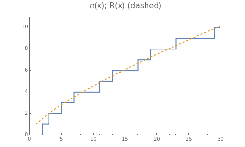
In number theory,

π(x)

is the number of primes less than or equal to

. Primes occur seemingly at random, so the graph of

π(x)

is quite irregular. This Demonstration shows how to use the zeros (roots) of the Riemann zeta function

ζ(s)

to get a smooth function that closely tracks the jumps and irregularities of

π(x)

. This illustrates the deep connection between the zeros of the zeta function and the distribution of primes.

Details

Snapshot 1: the graphs of

π(x)

and

R(x)

with no correction term

Snapshot 2: the graphs of

π(x)

and

R(x)

with correction term that uses the first 20 pairs of zeros of the zeta function

Snapshot 3: a closeup showing that

R(x)

with correction term correctly predicts the primes 103, 107, 109, 113, and 127, and the gap between 113 and 127; notice that, with no correction term,

R(x)

by itself misses these details

The function

π(x)

(Mathematica's built-in function PrimePi[x]) is a step function that jumps by 1 whenever

is prime. Riemann's prime-counting function

R(x)

(Mathematica's built-in function RiemannR[x]) is defined as

R(x)=

∞

∑

n=1

μ(n)

li(

1/n

)

where

μ(n)

is the Möbius mu function μ (MoebiusMu[n] in Mathematica) and

li(x)=

∫

log(t)

is the logarithmic integral (Mathematica's built-in function LogIntegral[x]).

Overall,

R(x)

is a good approximation to

π(x)

. However,

R(x)

does not track the details, that is, the jumps) of

π(x)

. Furthermore, when a gap occurs in the primes (as, for example, between 23 and 29),

R(x)

keeps increasing even though

π(x)

remains constant between primes.

However, if we add to

R(x)

a correction term that uses the first few zeros (roots) of the Riemann zeta function, something very surprising happens: we get a new function that very closely matches the jumps and irregularities of

π(x)

! When

is prime, this new function increases by about 1 near

, so, in effect, it "knows" where the primes are. And when a gap occurs, this new function tends to level out, again emulating the behavior of

π(x)

It's almost as if the zeros of the zeta function determine which numbers are prime!

The first three complex zeros of the zeta function are approximately

1/2+14.135i

1/2+21.022i

, and

1/2+25.011i

. The zeros occur in conjugate pairs, so if

a+bi

is a zero, then so is

a-bi

. The famous Riemann hypothesis is the claim that these complex zeros all have real part 1/2. All of the first

complex zeros do, indeed, have real part 1/2 (see[4]).

This Demonstration uses an exact formula for a function that is equal to

π(x)

except when

is prime. We define our new prime counting function, usually denoted by

(x)

, as follows. First, if

is a prime number, say,

, then

π(x)

jumps from

π(p)-1

π(p)

. For this

, we will define

(x)

to be halfway between these two values: that is,

(p)=π(p)-1/2

. Second, for all other values of

(x)=π(x)

. With this definition in mind,

(x)

has the following exact formula:

(1)

(x)=R(x)+

∞

∑

n=1

μ(n)

1/n

)

where

R(x)

is Riemann's prime counting function defined above, and

(2)

f(x)=-2Re

∞

∑

k=1

Ei(

log(x))+

∞

∫

(

-t)log(t)

dt-log(2)

where

is the

complex zero of the zeta function. In this formula,

Ei(z)

(Mathematica's built-in function ExpIntegralEi[z]) is the generalization of the logarithmic integral to complex numbers. These equations come from references[1],[2], and[3].

For a given

, and with the value of

that you choose with the slider control, here is how this Demonstration computes the correction term that involves zeta zeros:

First, let

be the smallest integer such that

1/M

. We need to add only the first

M-1

terms (that is,

n=1,2,…,M

) in the sum in equation (1). For each of these values of

, we use equation (2) to compute the value of

References:

[1] H. Riesel, Prime Numbers and Computer Methods for Factorization, 2nd ed., Boston: Birkhauser, 1994 pp. 44–55.
[2] H. Riesel and G Gohl, "Calculations Related to Riemann's Prime Number Formula," Mathematics of Computation, 24(112), 1970 pp. 969–983.
[3] S. Wagon, Mathematica in Action, 2nd ed., New York: Springer, 1999 pp. 540–554.
External Links
Permanent Citation
Robert Baillie