ABSTRACT (original article): Here we announce the construction and properties of a big commutative subalgebra of the Kirillov algebra attached to a finite dimensional irreducible representation of a complex semisimple Lie group. They are commutative finite flat algebras over the cohomology of the classifying space of the group. They are isomorphic with the equivariant intersection cohomology of affine Schubert varieties, endowing the latter with a new ring structure. Study of the finer aspects of the structure of the big algebras will also furnish the stalks of the intersection cohomology with ring structure, thus ringifying Lusztig’s q-weight multiplicity polynomials i.e., certain affine Kazhdan–Lusztig polynomials. CITATION (original article): Hausel, T. (2024). Commutative avatars of representations of semisimple Lie groups. In Proceedings of the National Academy of Sciences (Vol. 121, Issue 38). Proceedings of the National Academy of Sciences. https://doi.org/10.1073/pnas.2319341121
The Wolfram notebooks were prepared by Daniel Bedats.
For a finite dimensional irreducible representation of a complex semisimple Lie group G, the paper constructs a big algebra B, which is a commutative algebra, finite-free over a polynomial ring of invariant polynomials on the Lie algebra. This in particular means that the spectrum of the big algebra fibers over a vector space with finite fibers of constant length.
For example when G=SL_3 the coefficient ring is a polynomial ring generated by the Chern classes c2 and c3, which arise as the coefficients of the characteristic polynomial of a matrix in the lie algebra sl_3.
Examples of spectra of big algebras, their skeletons and principal spectra
Examples of spectra of big algebras, their skeletons and principal spectra
Standard representation of SL_3, Section 4.2.2. in the paper
Standard representation of SL_3, Section 4.2.2. in the paper
- Relation M1^3 + c2*M1 + c3 = 0 defines the big algebra
- Visualize real part of its spectrum, i.e. real vectors (c2, c3, M1) satisfying the relation
- Skeleton is restriction to c3 = 0
- Principal spectrum is restriction to c3 = 0, c2 = -4
Initial parameters:
c2max=5;c3max=5;m1max=3;thic=0.09;
Real spectrum of big algebra:
surface=ContourPlot3D[m1^3+c2*m1+c3==0,{c2,-c2max,c2max},{c3,-c3max,c3max},{m1,-m1max,m1max},PlotPoints->50,ContourStyle->Directive[Opacity[0.5],White],Extrusion->0.1,Mesh->None];
Skeleton equations:
Clear[c3];Solve[{m1^3+c2*m1+c3==0,c3==0},{c2,c3,m1}]
Out[]=
{{c2-,c30},{c30,m10}}
2
m1
Skeleton parametrization:
parabola=ParametricPlot3D[{-t^2,0,t},{t,-Sqrt[c2max],Sqrt[c2max]},PlotStyle->{Tube[thic],White}];line=ParametricPlot3D[{t,0,0},{t,-c2max,c2max},PlotStyle->{Tube[thic],White}];
Principal spectrum:
sol=Solve[{m1^3+m1*c2+c3==0,c3==0,c2==-4},{c2,c3,m1}];prinspec={c2,c3,m1}/.sol;bls=Graphics3D[{White,Sphere[prinspec,0.15]}];
In[]:=
Show[surface,parabola,line,bls,AxesLabel->{Subscript[c,2],Subscript[c,3],Subscript[m,1]},Lighting->"ThreePoint"]
Out[]=

The decuplet, the third symmetric power of the standard representation of SL_3, Section 4.2.3.
The decuplet, the third symmetric power of the standard representation of SL_3, Section 4.2.3.
- Full big algebra: coordinates (c2, c3, M1, M2) with two defining relations rel1, rel2 in the code
- Visualize real part of skeleton in coordinates (c2, M1, M2) by setting c3 = 0
- Principal spectrum is restriction of skeleton to c2 = -4
Compute the skeleton:
rel1=m1^4+4*c2*m1^2-6*m1^2*m2-6*c2*m2+3*m2^2-18*c3*m1;rel2=c2*m1^3+m1^3*m2+4*c2^2*m1+c2*m1*m2-3*m1*m2^2--c3*(3*m1^2-9*m2);c3=0;Solve[{rel1==0,rel2==0},{c2,m1,m2}]
Out[]=
c2,m10,{m10,m20},c2-,m20,{c2-,m2-},c2-,m2,{c2-,m2}
m2
2
2
m1
4
2
m1
2
m1
2
m1
9
2
m1
9
2
m1
2
m1
xmin=-5;xmax=1;ymin=-8;ymax=8;zmin=-12;zmax=8;
thic=0.063;
SKELETON consisting of parabolas and lines, rainbow colored:
p1=ParametricPlot3D[{t,0,0},{t,xmin,xmax},PlotStyle->{Tube[thic],Yellow},PlotRange->{{xmin,xmax},{ymin,ymax},{zmin,zmax}}];p2=ParametricPlot3D[{t,0,2*t},{t,xmin,xmax},PlotStyle->{Tube[thic],Blue},PlotRange->{{xmin,xmax},{ymin,ymax},{zmin,zmax}}];p3=ParametricPlot3D[{-t^2,t,-t^2},{t,-Sqrt[-xmin],Sqrt[-xmin]},PlotStyle->{Tube[thic],Cyan},PlotRange->{{xmin,xmax},{ymin,ymax},{zmin,zmax}}];p4=ParametricPlot3D[{-t^2,t,t^2},{t,-Sqrt[-xmin],Sqrt[-xmin]},PlotStyle->{Tube[thic],Orange},PlotRange->{{xmin,xmax},{ymin,ymax},{zmin,zmax}}];p5=ParametricPlot3D[{-t^2/9,t,t^2/9},{t,-3*Sqrt[-xmin],3*Sqrt[-xmin]},PlotStyle->{Tube[thic],Red},PlotRange->{{xmin,xmax},{ymin,ymax},{zmin,zmax}}];p6=ParametricPlot3D[{-t^2/4,t,0},{t,-2*Sqrt[-xmin],2*Sqrt[-xmin]},PlotStyle->{Tube[thic],Green},PlotRange->{{xmin,xmax},{ymin,ymax},{zmin,zmax}}];
skeleton=Show[p1,p2,p3,p4,p5,p6,AxesLabel->{Subscript[c,2],Subscript[m,1],Subscript[m,2]}]
Out[]=

Add principal spectrum:
dsol=Solve[{c2==-4,rel1==0,rel2==0},{c2,m1,m2}];dprinspec={c2,m1,m2}/.dsol;balls=Graphics3D[{White,Sphere[dprinspec,0.25]}];Show[skeleton,balls]
Out[]=

3D printed decuplet skeleton:
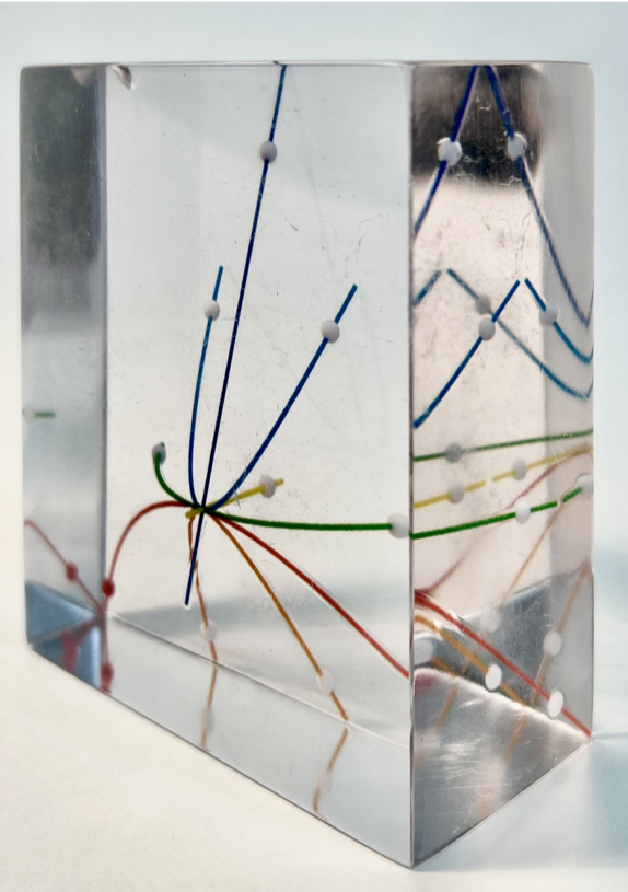
The octet, the adjoint representation of SL_3, Section 4.2.4.
The octet, the adjoint representation of SL_3, Section 4.2.4.
- Big algebra and medium algebra are distinct, equations in 4.2.4
- Big algebra in coordinates (c2,c3,M1,N1)
- Medium algebra in coordinates (c2,c3,M1,M2)
- Visualize big skeleton and medium skeleton by setting c3 = 0
- Here only the resulting parametrizations
White big skeleton, bp1 has a slightly different color - it is common to big and medium:
Light green medium skeleton:
Crystal graphs arising from big algebras
Crystal graphs arising from big algebras
One can draw the crystal graph of a big algebra, by the degeneration of the nerves to the so-called Levi walls and ordering the cluster of points in the principal spectrum which degenerate to the same point under this degeneration via their values on the M1 operator.
Example 1: Standard representation of SL_3
Example 1: Standard representation of SL_3
- Real spectrum of big algebra + skeleton + principal spectrum from above
- New: red and blue nerves and walls of the Weyl chamber
Walls of Weyl chamber:
Example 2: The decuplet
Example 2: The decuplet
- White skeleton + principal spectrum
- New: nerves and crystal graph
White SKELETON p1-p6:
Principal spectrum:
Blue nerve1 skeleton ner1-ner5:
Red nerve2 skeleton nerv1-nerv5:
Common part of both nerve skeleta is purple (blue & red mixed):
Crystal graph; blue and red parts; arrow = tube + cone:
3D printed decuplet crystal, skeleton and nerves:
Example 3 : The octet
Example 3 : The octet
- White big skeleton + big principal spectrum
- Red and blue nerves + crystal graph
White big skeleton:
Blue nerve1 skeleton:
Red nerve2 skeleton:
Purple common part of nerve1,2 skeleta:
Big octet with bigB = balls at its points:
Crystal graph:
CITE THIS NOTEBOOK
CITE THIS NOTEBOOK
Commutative avatars of representations of semisimple Lie groups
by Tamás Hausel and Daniel Bedats
Wolfram Community, STAFF PICKS, October 2, 2024
https://community.wolfram.com/groups/-/m/t/3290514
by Tamás Hausel and Daniel Bedats
Wolfram Community, STAFF PICKS, October 2, 2024
https://community.wolfram.com/groups/-/m/t/3290514