ABSTRACT (original article): Large primordial lepton flavor asymmetries with almost vanishing total baryon-minus-lepton number can evade the usual BBN and CMB constraints if neutrino oscillations lead to perfect flavor equilibration. Solving the momentum averaged quantum kinetic equations (QKEs) describing neutrino oscillations and interactions, we perform the first systematic investigation of this scenario, uncovering a rich flavor structure in stark contradiction to the assumption of simple flavor equilibration. We find (i) a particular direction in flavor space, for normal (inverted) neutrino mass hierarchy, in which the flavor equilibration is efficient and primordial asymmetries are essentially unconstrained, (ii) a minimal washout factor, yielding a conservative estimate for the allowed primordial asymmetries in a generic flavor direction, and (iii) particularly strong or weak washout if one of the initial flavor asymmetries vanishes due to non-adiabatic muon- or electron-driven MSW transitions. These results open up the possibility of a first-order QCD phase transition facilitated by large lepton asymmetries as well as baryogenesis from large and compensated asymmetries. Our systematic approach of deriving momentum averaged QKEs includes collision terms beyond the damping approximation, energy transfer between the neutrino and electron-photon plasma, and provides a fast and reliable way to investigate the impact of primordial lepton asymmetries at the time of BBN.We publicly release the Mathematica code COFLASY-M on https://github.com/mariofnavarro/COFLASY/ which solves the QKEs numerically. CITATION (original article): Domcke, V., Escudero, M., Navarro, M.F. et al. Lepton flavor asymmetries: from the early Universe to BBN. J. High Energ. Phys. 2025, 137 (2025). https://doi.org/10.1007/JHEP06(2025)137Valerie Domcke, Miguel Escudero, Mario Fernandez Navarro and Stefan Sandner (2025), A Limit on the Total Lepton Number in the Universe from BBN and the CMB, arXiv:2510.02438. https://doi.org/10.48550/arXiv.2510.02438
Δ≃-23 (-1)Δ
n
e
n
μ
Δ≤0.03 (0.016)Δ
2
n
e
|
BBN
∑
α
2
n
α
|
ini
Δ-Δ
n
e
n
μ
This code has been developed in order to study the evolution of primordial lepton flavour asymmetries from the early Universe to BBN, following the approach of arXiv:2502.14960. The GitHub repository of this code (https://github.com/mariofnavarro/COFLASY) consists of the following files:
BasicModule.m: contains all the definitions, equations and functions used to solve the system of differential equations and produce output.
COFLASY-M.nb: acts as the main front end notebook which loads BasicModule.m and contains a series of examples that serve as a tutorial for the user. These examples refer to some of the evolution plots in arXiv:2502.14960.
COFLASY-M.pdf: technical notes written in latex which contain a description of the full set of equations, definitions and functions that form the code.
BasicModule.nb: as of 07/10/2025, a .nb version of BasicModule.m has been added, which could be more clear for the user to modify.
To get started, we advise the user to read the technical notes (first part below). In order to run the code, the user may open the COFLASY-M.nb notebook and evaluate the “Basic module” section. Afterwards, the user may go through the “Examples” section in the COFLASY-M.nb notebook, which serves as a tutorial to get familiar with the code.
These technical notes describe the main features of COsmological evolution of FLavor ASYmmetries - Mathematica (COFLASY-M), a Mathematica code accompanying [1, 2]. The code numerically solves the quantum kinetic equations (QKEs) governing the evolution of primordial lepton asymmetries from the early Universe to BBN time. We refer the reader to [1] for a complete derivation of the equations and discussion of the dynamics of the system.
To use the code open the COFLASY-M.nb notebook and evaluate the “Basic module” section. Then you can go through the “Examples” section of the notebook, which serves as a tutorial for the user to get familiar with the code. In the following, we describe the sections contained in BasicModule.m, and at the end of this document we describe the output generated by the “Examples” section in the COFLASY-M.nb notebook.
Preliminaries
Preliminaries
In this section we define the following global constants: the reduced Planck mass , the Fermi constant , the W boson mass , the squared sine of the weak mixing angle , the electron and muon masses ,. We work in natural units and in MeV energy units by setting for all dimensionful quantities. We fix the values of the neutrino parameters () as in Appendix A of [1] and 0. All these parameters may be modified freely by the user. The code considers Normal neutrino mass hierarchy by default, but different values for (with opposite sign) and are provided for Inverted hierarchy.
M
P
G
F
M
ω
2
sin
θ
W
m
e
m
μ
MeV1
Δ,Δ,,,
2
m
21
2
m
31
θ
12
θ
13
θ
23
δ
CP
Δ
2
m
31
θ
23
We also define the Gell-Mann matrices , with , along with the structure constants of SU(3):
λ
i
i=1,...,8
ijk
f
1
4i
λ
i
λ
j
λ
k
(
1
)where and repeated indices are summed. Finally, we define the function gellMannComponents[X] which for any given 3 × 3 complex matrix returns its components in the basis formed by as a nine-dimensional vector, see Sec. IIC of [1] for more details.
i,j,k=1,...,8
(1,)
λ
i
Equations
Equations
The main goal of the code is to compute the evolution of the 3 × 3 neutrino and anti-neutrino density matrices in the presence of primordial asymmetries among neutrinos and anti-neutrinos, from the early Universe down to BBN times. We will work in the limit of neglecting the energy transfer among neutrinos and the cosmic plasma, which is achieved by imposing 1 in the equations derived in [1]. This limit is found to deliver accurate results for the evolution and asymptotic values of the neutrino flavor asymmetries, but does not allow for an accurate calculation of the effective number of relativistic degrees of freedom , as this crucially depends on the energy transfer rates that we are neglecting here. We refer the reader to [1] for further discussion.
z
ν
z
γ
N
eff
The neutrino and anti-neutrino density matrices and (T,k) are in general functions of both temperature and momentum . The crucial approximation of [1] is that we assume that the momentum dependence may be factored out from the temperature dependence as a Fermi-Dirac (FD) distribution without chemical potential following the temperature of the thermal plasma, i.e. our ansatz for the full density matrices in the limit 1 is:
ρ(T,k)
ρ
T
k
z
ν
z
γ
ρ(x,y)r(x)(y,0),(x,y)(x)(y,0),
f
fd
ρ
r
f
fd
(
2
)where we introduced the dimensionless variables and . is a reference temperature that may be fixed to any value, but a common convention is =. Given this ansatz, we can directly integrate the kinetic equations over momentum and solve for the temperature-dependent components and (x). In particular, the QKEs take the form:
x=/T
T
ref
y=k/T
T
ref
T
ref
m
e
r(x)
r
Hx=-i[〈〉+〈〉+〈〉(r-),r]+〈ℐ〉,Hx=+i[〈〉+〈〉-〈〉(r-),]+〈〉,
′
r
H
0
V
c
V
s
r
′
r
H
0
V
c
V
s
r
r
ℐ
(
3
)where we denote . The Hubble parameter is given by:
′
∂
x
H
H(x).
g
*
2
π
90
M
P
2
T
ref
x
(
4
)In the limit 1, the effective number of degrees of freedom (x) under the approximation (2) is estimated as:
z
ν
z
γ
g
*
g
*
γ
g
*
±
e
g
*
ν
g
*
7
8
7
8
r
(
5
)In all cases, denotes momentum average and we work in the flavor basis. We refer the reader to Sec. II of [1] for the derivation of the equations and for a complete discussion and description of each term. In the following we write each contribution in the limit 1. The vacuum Hamiltonian contribution is given by:
〈...〉
z
ν
z
γ
〈〉U,
ℋ
0
x
T
ref
2
π
36ζ(3)
2
M
†
U
(
6
)where diag0,Δ,Δ and is the PMNS matrix, where we follow the PDG convention. The matter potentials contribute as:
2
M
2
m
21
2
m
31
U
〈〉-2(+),
V
c
2
7
4
π
180ζ(3)
G
F
2
M
W
5
T
ref
x
(
7
)〈〉,
V
s
3
2
2
G
F
ζ(3)
2
π
3
T
ref
x
(
8
)where is a diagonal matrix in flavor space encoding the dimensionless energy and pressure densities of charged leptons and anti-leptons, and it is well approximated by:
(+)
(+)
ee
7
2
π
45
1
6
2
2
m
e
x
T
ref
(
9
)(+)
μμ
2
2
π
3
3
m
μ
x
T
ref
K
3
m
μ
x
T
ref
(
10
)where denotes the modified Bessel function of second kind. For the component we can safely assume =0.
K
i
τ
(+)
τ
For the rest of technical notes please see the file COFLASY-M.pdf in https://github.com/mariofnavarro/COFLASY/
Basic instructions
Basic instructions
The code works as follows:
1
.Evaluate the “Basic module” section.
2
.The “Examples” section serves as a tutorial to use the code and generates some of the plots in [2502.14960]. Evaluating the full section may take around 15 min, some examples take only a few seconds while others take several minutes.
Basic module
Basic module
Load the basic module which contains all equations and functions to solve the system, takes around 10 seconds
ClearAll["Global`*"](*Toclearyourkernelbeforeloadingthebasicmodule*)ClearSystemCache[]SetDirectory[NotebookDirectory[]];Get["BasicModule.m"]
Examples
Examples
Benchmarks of the paper with FD collisions
Benchmarks of the paper with FD collisions
We provide initial conditions over (A, ϕ)
Aval=0.01;ϕval=;
π
3
We translate from (A, ϕ) to (ξe, ξμ, ξτ), alternatively the user may provide conditions over (ξe, ξμ, ξτ) directly
ξeini=ξtildetoξ[ξtile[Aval,ϕval]];ξμini=ξtildetoξ[ξtilμ[Aval,ϕval]];ξτini=ξtildetoξ[ξtilτ[Aval,ϕval]];
This is the minimum input required to run the solving functions, with all the optional arguments using default values
We run the system with FD collisions
We run the system with FD collisions
Fig5aFD=solveFD[ξeini,ξμini,ξτini]
Starting evolution of the full system
System evolved until =1.5 MeV
T
ave
Final ξe: 0.000213501
Thermodynamics are output to: output/output.dat
Total execution time: 6.901s
Out[]=
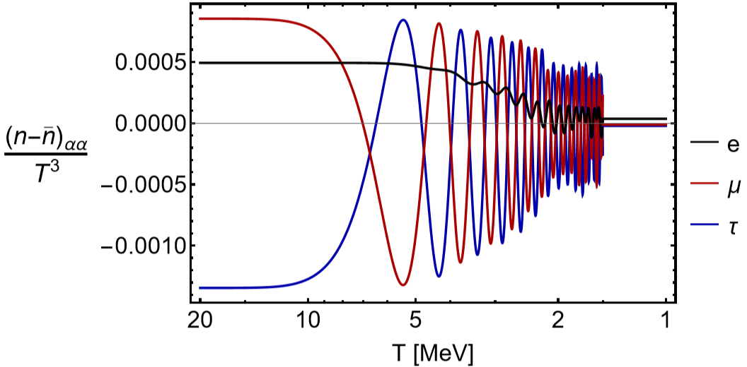
Alternatively, the user can define all the optional arguments to be used by the solving functions
As optional arguments, we provide a name for the .dat file containing the output (filename), initial temperature (Tini), temperature at which oscillation average is taken (Tave), and we extend asymptotically the result at Tave until a final temperature (Tfinal).
Note we must provide Tini < Tave <= Tfinal for consistency.
We also provide accuracy (accval) and precision (precval) settings for NDSolve. The solving method (solverMethod) used by NDSolve may also be specified.
adiabatic->False runs the full system, while adiabatic->True runs the system in the adiabatic approximationw where Vs=0. Finally,timeoutAdiabatic is the execution time in seconds after which the solver switches to the adiabatic approximation, useful for numerically challenging benchmarks.
This benchmark is more numerically challenging and the solver gets stuck around T = 2 MeV, but fortunately the timeout switches to adiabatic and allows to reach Tave = 1.5 MeV
Benchmarks of the paper with collision terms in the damping approximation
Benchmarks of the paper with collision terms in the damping approximation
Running in the damping approximation is typically much faster
The function solveDamping receives the same arguments as solveFD
The next two benchmarks work better with StiffnessSwitching than with BDF
References
References
[1] V. Domcke, M. Escudero, M. Fernandez Navarro, and S. Sandner, Lepton flavor asymmetries: from the early Universe to BBN, JHEP 06, 137, arXiv:2502.14960 [hep-ph].
[2] V. Domcke, M. Escudero, M. Fernandez Navarro, and S. Sandner, A Limit on the Total Lepton Number in the Universe from BBN and the CMB, (2025), arXiv:2510.02438 [hep-ph].
[3] J. Froustey and C. Pitrou, Primordial neutrino asymmetry evolution with full mean-field effects and collisions, JCAP 03 (03), 065, arXiv:2110.11889 [hep-ph].
CITE THIS NOTEBOOK
CITE THIS NOTEBOOK
A limit on the total lepton number in the universe from BBN and the CMB
by Valerie Domcke, Miguel Escudero, Mario Fernandez Navarro & Stefan Sandner
Wolfram Community, STAFF PICKS, January 29, 2026
https://community.wolfram.com/groups/-/m/t/3630958
by Valerie Domcke, Miguel Escudero, Mario Fernandez Navarro & Stefan Sandner
Wolfram Community, STAFF PICKS, January 29, 2026
https://community.wolfram.com/groups/-/m/t/3630958