We discussed how a spin system in a time-dependent magnetic field accumulates both a dynamical phase and a geometric (Berry) phase during its evolution. The geometric phase depends solely on the path taken by the magnetic field’s direction and is related to the solid angle that the path subtends. A key point was that the standard eigenstates are not single‑valued when the azimuthal angle wraps around, so a gauge transformation is applied to make them single‑valued, which then correctly accounts for the extra phase.
In[]:=
PacletInstall[CloudObject["https://wolfr.am/DevWQCF"],ForceVersionInstall->True]<<Wolfram`QuantumFramework`
Out[]=
PacletObject

Consider a spin- system (which is in dimensional Hilbert space):
j
2j+1
In[]:=
j=7/2;
Consider Hamiltonian as where is the angular momentum operator and is an externally controlled magnetic field with a fixed magnitude but a direction given by polar angle: =B{Cos[ϕ[t]]Sin[θ[t]],Sin[θ[t]]Sin[ϕ[t]],Cos[θ[t]]}
H=.
B(t)
J
J
B(t)
B(t)
Construct the Hamiltonian:
In[]:=
$Assumptions={θ[t],ϕ[t]}∈Reals;hamiltonian=FromSphericalCoordinates[{1,θ[t],ϕ[t]}].Table[QuantumOperator[st[j]]["Computational"]["Matrix"],{st,{"JX","JY","JZ"}}];
Show eigenvalues:
In[]:=
Eigenvalues[hamiltonian]
Out[]=
-,,-,,-,,-,
7
2
7
2
5
2
5
2
3
2
3
2
1
2
1
2
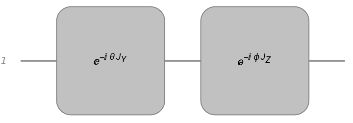
Given the position in the parameter space, it can be described as a rotation around y-axis followed by a rotation around z-axis:
In[]:=
rot=QuantumCircuitOperator{"R",2theta,QuantumOperator["JY"[j]]}->"Label"->"",{"R",2phi,QuantumOperator["JZ"[j]]}->"Label"->"","Parameters"->{theta,phi};rot["Diagram"]
-θ
J
Y
-ϕ
J
Z
Out[]=
Show |j,m〉 are eigenstates of Hamiltonian with the eigenvalue :
-ϕ
J
Z
-θ
J
Y
m
In[]:=
With[{sv=rot[<|theta->θ[t],phi->ϕ[t]|>][#]["Computational"]["StateVector"]},Conjugate[sv].hamiltonian.sv]&/@QuantumBasis["JZ"[j]]["BasisStates"]//FullSimplify
Out[]=
-,-,-,-,,,,
7
2
5
2
3
2
1
2
1
2
3
2
5
2
7
2
Note that parameters ϕ and θ are time-dependent. Therefore, |j,m〉 are the instantaneous eigenstates of Hamiltonian at a given time.
-ϕ
J
Z
-θ
J
Y
Generate the instantaneous eigenstates, (θ,ϕ), in the direction specified by θ(t) and ϕ(t):
ψ
m
In[]:=
instantaneousEigenstates=rot[<|theta->θ[t],phi->ϕ[t]|>]/@QuantumBasis["JZ"[j]]["BasisStates"]//FullSimplify;
Calculate Berry connection, =, in the direction of ϕ:
ϕ
ψ
m
∂
ϕ
ψ
m
In[]:=
Conjugate[#["StateVector"]].D[Normal@#["StateVector"],ϕ[t]]&/@instantaneousEigenstates//FullSimplify
Out[]=
-Cos[θ[t]],-Cos[θ[t]],-Cos[θ[t]],-Cos[θ[t]],Cos[θ[t]],Cos[θ[t]],Cos[θ[t]],Cos[θ[t]]
7
2
5
2
3
2
1
2
1
2
3
2
5
2
7
2
Calculate Berry connection, =〈|〉, in the direction of θ:
θ
ψ
m
∂
θ
ψ
m
In[]:=
Conjugate[#["StateVector"]].D[Normal@#["StateVector"],θ[t]]&/@instantaneousEigenstates//FullSimplify
Out[]=
{0,0,0,0,0,0,0,0}
Berry phase requires that the eigenstates be chosen in a single‑valued gauge. For this aim, when , in the rotation operator, we will have an additional term which introduces an overall phase :j,m=()|j,m〉=|j,m〉=j,m
ϕ->ϕ+2π
-2π
J
z
-2πm
-2π
J
z
-ϕ
J
Z
-θ
J
Y
-ϕ
J
Z
-2π
J
z
-θ
J
Y
2π
J
z
-2π
J
z
-ϕ
J
Z
-θ
J
Y
-2π
J
z
-2πm
-ϕ
J
Z
-θ
J
Y
An overall phase means the state is not strictly identical to its starting value. We can redefine the eigenstate by absorbing a compensating phase factor so that the state does not change (up to a physically irrelevant overall phase) when ϕ goes from 0 to 2π.
-2πm
In[]:=
instantaneousEigenstates=Table[Exp[mϕ[t]],{m,-j,j}]instantaneousEigenstates//FullSimplify;
Calculate Berry connection, =, in the direction of ϕ (the expected result is =m(-1+Cos[θ])):
ϕ
ψ
m
∂
ϕ
ψ
m
ϕ
In[]:=
Conjugate[#["StateVector"]].D[Normal@#["StateVector"],ϕ[t]]&/@instantaneousEigenstates//FullSimplify//TrigReduce
Out[]=
-(-1+Cos[θ[t]]),-(-1+Cos[θ[t]]),-(-1+Cos[θ[t]]),(1-Cos[θ[t]]),(-1+Cos[θ[t]]),(-1+Cos[θ[t]]),(-1+Cos[θ[t]]),(-1+Cos[θ[t]])
7
2
5
2
3
2
1
2
1
2
3
2
5
2
7
2
Calculate Berry connection, =〈|〉, in the direction of θ (the expected result is =0)
θ
ψ
m
∂
θ
ψ
m
θ
In[]:=
Conjugate[#["StateVector"]].D[Normal@#["StateVector"],θ[t]]&/@instantaneousEigenstates//FullSimplify//TrigReduce
Out[]=
{0,0,0,0,0,0,0,0}
Now consider the following case: with and . In this case, the field rotates at a constant angular speed ω while the polar angle θ remains fixed.
ϕ(t)=ωt
ω≪1
θ(t)=
θ
0
B(t)
In[]:=
ω=.01;θ0=π/3;hamiltonian={Cos[tω]Sin[θ0],Sin[θ0]Sin[tω],Cos[θ0]}.Table[QuantumOperator[st[j]]["Computational"]["Matrix"],{st,{"JX","JY","JZ"}}];
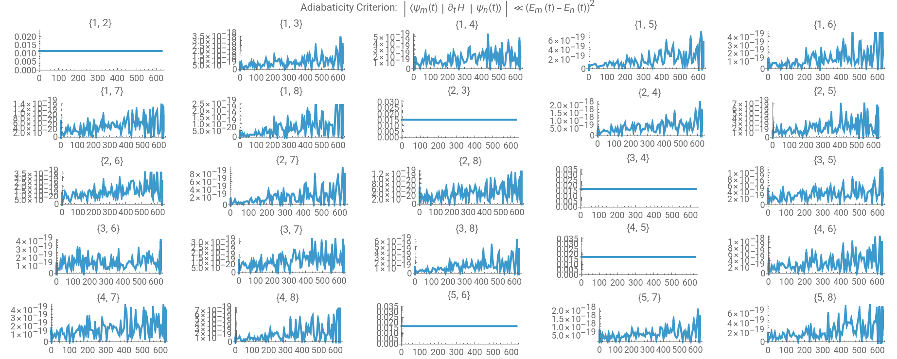
In this setup, we will first check for Adiabaticity Criterion. A rough estimate of the adiabaticity condition is given by: for . This condition is our case will be of the order of ω.
≪1
〈(t)|H|(t)〉
ψ
m
∂
t
ψ
n
2
((t)-(t))
E
m
E
n
m!=n
In[]:=
Module{dotH,stateVectors,adiabatic},dotH=D[hamiltonian,t];stateVectors=FullSimplify[Normal[#["Computational"]["StateVector"]]/.{θ[t]->θ0,ϕ[t]->ωt}]&/@instantaneousEigenstates;adiabatic=FlattenTablesvM1,svM2,Abs,{svM1,Length@stateVectors},{svM2,svM1+1,Length@stateVectors},1;ShowGraphicsGrid[Partition[Plot[#3,{t,0,2π/ω},PlotLabel->{#1,#2},PlotPoints->100,AspectRatio->1/3]&@@@adiabatic,5],Spacings->0,ImageSize->Full],PlotLabel->"Adiabaticity Criterion: (t)H(t)≪"
Conjugate[stateVectors[[svM2]]].dotH.stateVectors[[svM1]]
2
(svM1-svM2)
ψ
m
∂
t
ψ
n
2
((t)-(t))
E
m
E
n
Out[]=
Under the adiabatic assumption, one neglects off-diagonal couplings in the instantaneous basis. The state then evolves simply as where the phase is given by (t)=+ with =-mt the dynamical phase, and the geometric phase which depends on Berry connections =ϕ+θ. Note in our case, we have =-m(1-Cos[]) and =0. Therefore, the geometric phase is given by =-mΔϕ(1-Cos[]). If we consider a loop in the parameter space, , then we find =-2πm(1-Cos[]).
|ψ(t)〉≈|(θ,ϕ)〉
(t)
Φ
m
ψ
m
Φ
m
Φ
dyn
Φ
geo
Φ
dyn
Φ
geo
Φ
geo
ϕ
f
∫
ϕ
i
ϕ
θ
f
∫
θ
i
θ
ϕ
θ
0
θ
Φ
geo
θ
0
Δϕ=2π
Φ
geo
θ
0
We now simulate the evolution starting from an initial state, and compare the phase induced.
Define Hamiltonian operator:
In[]:=
hamiltonianOperator=QuantumOperator[hamiltonian,2j+1]
Out[]=
QuantumOperator

Define initial state (as a instantaneous state at time )
t=0
In[]:=
m=-3/2;initialState=rot[<|theta->θ0,phi->0|>]@QuantumState[ToString[m+j],"JZ"[j]]//N
Out[]=
QuantumState

Find the final state through time evolution (note the Hamiltonian is time dependent, and does not commute in different times):
In[]:=
finalState=QuantumEvolve[hamiltonianOperator,initialState,{t,0,tf=2π/ω}]
Out[]=
QuantumState

Since we want to check , construct the state. Create the state vector of desired instantaneous eigenstate:
|ψ(t)〉≈|(θ,ϕ)〉
(t)
Φ
m
ψ
m
|(θ,ϕ)〉=|j,m〉
ψ
m
-ϕ(t)
J
Z
-
θ
0
J
Y
In[]:=
target=FullSimplify[Normal[rot[<|theta->θ0,phi->ωt|>][Exp[ωtQuantumOperator["JZ"[j]]][QuantumState[ToString[m+j],"JZ"[j]]]]["Computational"]["StateVector"]]]//N;
Find the inner product :
〈(θ,ϕ)|ψ(t)〉
ψ
m
In[]:=
inner=Conjugate[target].finalState[t]["Computational"]["StateVector"];
Plot the absolute value of the inner product (we expect it to be very close to 1):
In[]:=
Plot[Abs@inner,{t,0,tf},Exclusions->None,GridLines->Automatic,AspectRatio->1/2,AxesLabel->{"Time","Abs[〈(θ,ϕ)|ψ(t)〉]"},PlotLabel->"Magnitude of the inner product between the instantaneous eigenstate\n and the state obtained via time evolution at time t"]
ψ
m
In numerical simulations, the phase is usually reported within a specific interval (commonly between -π and π) to avoid discontinuities. However, the analytical formula might yield a phase outside this range. To compare them meaningfully, you need to “wrap” the analytical phase into the same interval, ensuring that any apparent differences are not just due to the periodic nature of the phase but reflect the true physical behavior.
Plot the argument of the inner product and compare it with the analytical formula:
We can also show that the difference of numerical calculation of the phase and the analytical formula (from adiabatic approximation) is very small.
CITE THIS NOTEBOOK
CITE THIS NOTEBOOK
Geometric phase (Berry phase) for spin systems
by Mohammad Bahrami
Wolfram Community, STAFF PICKS, March 26, 2025
https://community.wolfram.com/groups/-/m/t/3432889
by Mohammad Bahrami
Wolfram Community, STAFF PICKS, March 26, 2025
https://community.wolfram.com/groups/-/m/t/3432889