A polynomial with a single variable must always yield either be a finite set, or a simple polynomial progression of values. The goal of this paper is to initiate thought in finding a diophatine equation that produces positive integer solutions to y-xand . Although this essay does not provide the exact solution as it has been unsolved till date, it shows multiple interpretations of the question and some results and theory that back it.
2
x
3
y
x+1
2
y
Introduction
Introduction
In this essay, we explore various polynomials and their value sets to see if we can model a diophantine equation after it. I have explored the polynomials y-x and . To begin, I started by analyzing the infamous polynomial +xy±1 which have solutions as Fibonacci[n, n-1]. I generalized that polynomial to +axy+bk and played around with some of the properties of the cardinality of the set under a finite field. I then moved on to observing the solutions of y-x in the finite field and enumerated fibonacci-related polynomials to see if any pattern or generalization show up. Finally, I found some fibonacci solutions in the value set of .
2
x
3
y
x+1
2
y
2
x
2
y
{x,y}
2
x
2
y
2
x
3
y
x+1
2
y
Proof of the cardinality of the set of solutions of 2x+axy+b2yk over a finite field
Proof of the cardinality of the set of solutions of +axy+bk over a finite field
2
x
2
y
Background
Background
A finite field is a finite set that is a field(multiplication, addition, subtraction and division (excluding division by zero) are defined and satisfy the rules of arithmetic). The number of elements of a finite field is called its order or size. A finite field of order exists if and only if is a prime power (where is a prime number and is a positive integer).
q
q
k
p
p
k
Statement
Statement
In this subsection, I am going to sketch a proof of the formula for the cardinality of the set of solutions of +axy±1 over a finite field. I have also created a function to help generate the cardinality. The cardinality of the set is if p divides and 1 and the cardinality of the set is if p does not divide . An extension is that the cardinality of the set is 0 if -1 but we won’t explore that case since we are only looking at positive integer solutions.
2
x
2
y
2p
4b-
2
a
k
p
p--4b
2
a
p
4b-
2
a
k
p
Sketch of proof
Sketch of proof
Case 1: mod then 4k If -1, then +axy+bk has no solutions.If 1, then in mod for some n such that 4k For each , there are two such . Therefore for each there are two corresponding to . Hence there are solutions.
(4b-)≡0
2
a
p
2
(2x+ay)
k
p
2
x
2
y
k
p
2x+ay≡±n
p
2
n
k
n
y
x
y
2p
Function
Function
I have simulated this property of set of solutions of +axy+bk using a function.
2
x
2
y
In[]:=
CardinalityOfSetOfSolutions[poly_,prime_]:=Module[{a,b,k,discriminant},a=ToExpression[StringTake[StringCases[poly,__~~"x"~~"y"],1]];b=ToExpression[StringTake[StringCases[poly,__~~"y^2"],1]];k=ToExpression[StringTake[StringCases[poly,"=_"],{2}]];discriminant=4*b-a^2;If[Mod[prime,discriminant]==0&&Mod[k,prime]==1,2*prime,prime-(a^2-4*b)/prime]]
Geometric interpretation of diophantine equations
Geometric interpretation of diophantine equations
The problem closely related to this is solving Diophantine equations. A Diophantine equation is an equation, typically a polynomial equation in two or more unknowns with integer coefficients, for which only integer solutions are of interest. There are various types of Diophantine equation: linear and exponential. A linear Diophantine is an equation that a constant the sum of two or more monomials, each of degree one. An exponential Diophantine equation is one in which unknowns can appear in exponents. There are geometric interpretations of diophatine equations too. Solving Diophantine equations often reduces to studying rational points on their respective curve representation. A point is a rational point if the coordinates x, y are rational numbers. Additionally, if satisfy for some , we call rational solutions to . We can learn how genus correlates with the number of solutions. A genus of a graph. is the minimum number of handles that must be added to the plane to embed the graph without any crossings. Smooth curves of genus 0 are given by polynomial equations of degree1 or 2, namely lines and conics. Pell equations are smooth curves with genus 0 and degree 2. -d1 is a Pell-equation where where d ∈ N and where d is not a perfect square. All positive solutions (,) of -d1 are given by +Since we can take k to be any power, the Pell equation has infinitely many integer solutions. Hence we have some evidence that non-singular genus 0 curves have might infinitely many rational solutions. It turns out that C(Q) which is the set of all rational points on a curve C have either infinite solutions or no solutions.
(x,y)
x,y
f(x,y)0
f
x,y
f
2
x
2
y
x
k
y
k
2
x
2
y
x
k
d
y
k
k
+
x
1
d
y
1
This is an example of a Pell equation -21
2
x
2
y
eq=x^2-2y^2==1;ContourPlot[eq,{x,-3,3},{y,-2,2},PlotLegends->None,ContourStyle->{Thick,Blue},AxesLabel->{"x","y"},PlotRange->{{-3,3},{-2,2}}GridLines->Automatic,Frame->True,FrameLabel->{"x","y"},AxesOrigin->{0,0},Epilog->{Red,PointSize[Medium],Point[{{1,0},{-1,0},{3,1},{-3,-1},{3,-1},{-3,1}}]}]integerSolutions={{1,0},{-1,0},{3,1},{-3,-1},{3,-1},{-3,1}};
Out[]=
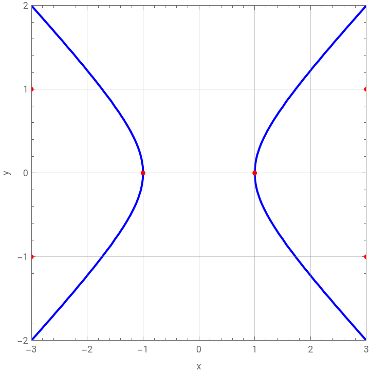
This helps us analyze the number of solutions of any diophantine equation and can be useful to understand the value set of the polynomials better.
Initial stages
Initial stages
To tackle the actual problem, I first tried to plot the solutions of y-x on a finite field to see any patterns
2
x
3
y
In[]:=
ℱ=FiniteField[11];primes=Map[#["Index"]&,{x,y}/.{Reduce[x^2-x*y^3==1,{x,y},ℱ]//ToRules},{2}]points=primes/.{{a_,b_}:>{a,b}};primeList=Prime[Range[1,200]];Manipulate[Module[{currentField,fieldPoints},currentField=FiniteField[prime];fieldPoints=Map[#["Index"]&,{x,y}/.{Reduce[x^2-x*y^3==1,{x,y},currentField]//ToRules},{2}];fieldPoints=fieldPoints/.{{a_,b_}:>{a,b}};ListPlot[fieldPoints,PlotStyle->Red]],{{prime,11,"Prime for Finite Field"},primeList,ControlType->PopupMenu}]
Out[]=
{{1,0},{2,6},{3,10},{4,1},{5,6},{6,5},{7,10},{8,1},{9,5},{10,0}}
Out[]=

In[]:=
ℱ=FiniteField[11];primes=Map[#["Index"]&,{x,y}/.{Reduce[x^2-x*y^3==1,{x,y},ℱ]//ToRules},{2}]points=primes/.{{a_,b_}:>{a,b}};labels=CharacterRange["A","Z"];labels=Take[labels,Length[points]];offset={0.2,0.2};ListPlot[points,PlotStyle->Red,Epilog->(Text[Style[labels[[#]],Black,12],points[[#]]+offset]&/@Range[Length[points]])]
The finite field with prime 11 is interesting for the following reasons:
- the slope of BD = GI is 4 and the slope of BC = HI is 2.5
- BD = GI
- BC = HI
- CG = DH
- the slope of BD = GI is 4 and the slope of BC = HI is 2.5
- BD = GI
- BC = HI
- CG = DH
Maltese cross curves
Maltese cross curves
Background
Background
this is the polynomial x^2y-xy^3
this is the maltese cross curve
this is the polynomial x^2y-xy^3
this is the maltese cross curve
Bonus (Just a spiel on how to recover “lost” points from intersections of algebraic curves)
Bonus (Just a spiel on how to recover “lost” points from intersections of algebraic curves)
Computations
Computations
My first approach with everything I explored above was to find existing theorems and properties of curves that might direct us to the value set. My second approach here was to just compute various polynomials to see if anything interesting pops up.
Leads
Leads
The Reduce function gives us some equations to manipulate.
Visualizations
Visualizations
These are a few visualizations which help us understand our polynomials better
Extensions
Extensions
We can take this information and experiment in many ways: more manipulation of fibonacci equations, more exploration of algebraic curves relating to it and exploring solutions in the finite field. In the future I would like to add some more cool visualizations and take a geometric approach. It is also feasible to convert the question into finding the rational points of the corresponding projective hypersurface. Minkowski’s First theorem might also hint at possible solutions.
Conclusion
Conclusion
Although this problem is very out of reach for its erratic behaviors with no sense of patterns that stand out, we can definitely further research in this area by having an interdisciplinary approach by combining algebra and geometry. Thinking about this simply as a diophatine might limit us to certain avenues but expanding our horizons with geometry might lead us to some more prospects. Also incorporating fibonacci arguments (Cassini’s identity) could also be helpful.
References
References
SUPAWADEE Prugsapitak Prince of songkla university. (n.d.). https://www.researchgate.net/profile/Supawadee_Prugsapitak
Kendig, K. (n.d.). In A Guide to Plane Algebraic Curves. essay.
Cassini’s identity. ProofWiki. (n.d.). https://www.proofwiki.org/wiki/Cassini%27s_Identity
Rational points on curves. (n.d.-a). https://sites.math.washington.edu/~morrow/336_20/papers18/blanca.pdf
Kendig, K. (n.d.). In A Guide to Plane Algebraic Curves. essay.
Cassini’s identity. ProofWiki. (n.d.). https://www.proofwiki.org/wiki/Cassini%27s_Identity
Rational points on curves. (n.d.-a). https://sites.math.washington.edu/~morrow/336_20/papers18/blanca.pdf
Acknowledgements
Acknowledgements
I would like to thank my mentor Macy Levin and Rockstar the energy drink.
CITE THIS NOTEBOOK
CITE THIS NOTEBOOK
Polynomial value sets of various polynomials
by Sahiti Doke
Wolfram Community, STAFF PICKS, July 11, 2024
https://community.wolfram.com/groups/-/m/t/3217257
by Sahiti Doke
Wolfram Community, STAFF PICKS, July 11, 2024
https://community.wolfram.com/groups/-/m/t/3217257