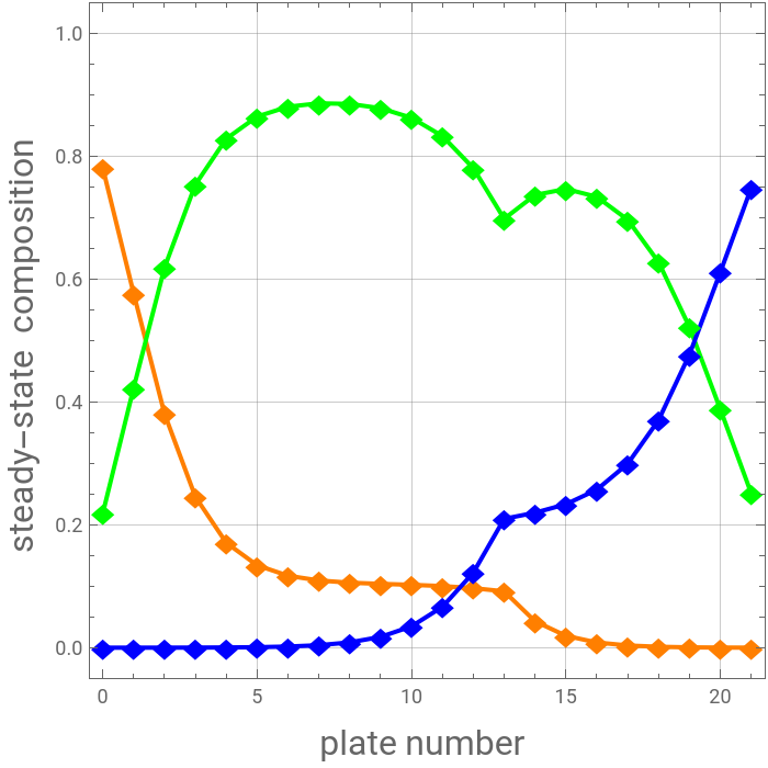
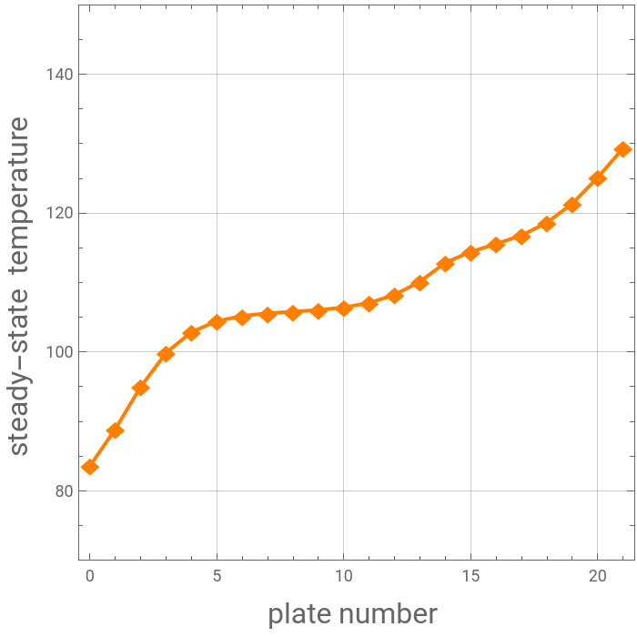
Consider a distillation column operating at 101.325 kPa and separating an equimolar mixture of benzene (), toluene (), and -xylene (). The column has 20 stages, a partial reboiler, and a total condenser. The feed location is stage 13 counting from the top. The feed, a saturated liquid, has a flow rate equal to 100 kmole/hr. The column has a liquid sidestream at stage 7 counting from the top. You can set the draw rate of this side-stream as well as the reflux and reboil ratios of the column. The We plots the composition profile in orange, green, and blue for benzene, toluene, and -xylene, respectively. Plots of the temperature profile and liquid and vapor flow rates are also given. The variables , , , and stand for feed, distillate, residue, and sidestream flow rates, respectively. The column’s degree of freedom is 3 and we choose to fix: the reflux ratio, the reboil ratio and the sidestream draw rate. Finally, we compare with the results of PYTHON and provide the corresponding PYTHON coding.
B
T
p
X
p
F
D
R
S
In[]:=
Srate=15;RReflux=5;RReboil=5;(*ModifiedAntoineConstantsforBenzene-toluene-p-xylenereproducedfromAspen-HYSYS*)A1=169.65;B1=-10314.8;C1=0.;D1=-23.5895;E1=;F1=2.;A2=76.4511;B2=-6995.;C2=0.;D2=-9.1635;E2=;F2=2.;A3=91.2505;B3=-8121.25;C3=0.;D3=-11.3188;E3=;F3=2.;PSat[1][i_]:=/.TT[i];PSat[2][i_]:=/.TT[i];PSat[3][i_]:=/.TT[i];
2.09442
5
10
6.225
6
10
7.30555
6
10
E1+A1+D1Log[T]+
F1
T
B1
C1+T
E2+A2+D2Log[T]+
F2
T
B2
C2+T
E3+A3+D3Log[T]+
F3
T
B3
C3+T
Constants for liquid and vapor enthalpies for Benzene - toluene - p-xylene reproduced from Aspen-HYSYS
a1=0.;b1=129.44;c1=-;d1=;e1=-;h1=e1+d1+c1+b1T+a1/.TTF;hl1=e1+d1+c1+b1T+a1-h1;a2=0.;b2=140.1399;c2=-;d2=;e2=-;h2=e2+d2+c2+b2T+a2/.TTF;hl2=e2+d2+c2+b2T+a2-h2;a3=0.;b3=-35.49996;c3=0.6435998;d3=-;e3=;h3=e3+d3+c3+b3T+a3/.TTF;hl3=e3+d3+c3+b3T+a3-h3;a1v=45880.06;b1v=114.7825;c1v=-0.2426732;d1v=;e1v=-;Hv1=e1v+d1v+c1v+b1vT+a1v-h1;a2v=48522.49;b2v=132.693;c2v=-0.2388932;d2v=;e2v=-;Hv2=e2v+d2v+c2v+b2vT+a2v-h2;a3v=11653.17;b3v=383.7983;c3v=-1.17436;d3v=;e3v=-;Hv3=e3v+d3v+c3v+b3vT+a3v-h3;
8.475001
2
10
2.159366
4
10
2.089645
14
10
4
T
3
T
2
T
4
T
3
T
2
T
7.615016
2
10
2.31667
4
10
2.769433
14
10
4
T
3
T
2
T
4
T
3
T
2
T
8.66333
4
10
6.064997
7
10
4
T
3
T
2
T
4
T
3
T
2
T
5.663124
4
10
3.654795
7
10
4
T
3
T
2
T
5.907287
4
10
3.913967
7
10
4
T
3
T
2
T
2.308164
3
10
1.543837
6
10
4
T
3
T
2
T
Liquid\b-phase and vapor-phase enthalpies for mixtures of Benzene - toluene - p-xylene
H[i_]:=Hv1y[1][i]+Hv2y[2][i]+Hv3y[3][i]/.TT[i];h[i_]:=hl1x[1][i]+hl2x[2][i]+hl3x[3][i]/.TT[i];
Feed thermal quality and composition
z[i_]:=1/3;phi=0;
Total pressure
P=101.325;
Some calculation regarding the feed stream
solf=QuietFindRoot0,{T[1],350,420};TF=T[1]/.solf(*feedstreamtemeprature*)hF=(1-phi)(hl1xz[1]+hl2xz[2]+hl3xz[3])+phi(Hv1yz[1]+Hv2yz[2]+Hv3yz[3])/.TTF;(*feedstreamentahlpy*)hF(*vaporinequilibrium---itscomposition*)yz[1]=/.solf;yz[2]=/.solf;yz[3]=/.solf;yz[4]=/.solf;(*liquidinequilibrium---itscomposition*)xz[1]=/.solf;xz[2]=/.solf;xz[3]=/.solf;xz[4]=/.solf;Table[xz[i],{i,1,3}]Table[yz[i],{i,1,3}]
3
∑
i=1
-1z[i]
PSat[i][1]
P
-1phi+1
PSat[i][1]
P
PSat[1][1]xz[1]
P
PSat[2][1]xz[2]
P
PSat[3][1]xz[3]
P
PSat[4][1]xz[4]
P
z[1]
-1phi+1
PSat[1][1]
P
z[2]
-1phi+1
PSat[2][1]
P
z[3]
-1phi+1
PSat[3][1]
P
z[4]
-1phi+1
PSat[4][1]
P
Out[]=
374.497
Out[]=
3.03165×
-12
10
Out[]=
,,
1
3
1
3
1
3
Out[]=
{0.634953,0.254035,0.111012}
Summation rules
y[3][i_]:=-y[1][i]-y[2][i]+1;x[3][i_]:=-x[1][i]-x[2][i]+1;
Feed flow-rate
F=100;(*MESHEquations*)eq1=Di+L[0]V[1];eq2=Dih[0]+L[0]h[0]V[1]H[1]+Qc;eq3[i_]:=V[i]+L[i]+If[i7,S,0]If[i13,F,0]+V[i+1]+L[i-1];eq4[i_]:=Table[V[i]y[j][i]+L[i]x[j][i]+If[i7,Sx[j][i],0]If[i13,Fz[j],0]+V[i+1]y[j][i+1]+L[i-1]x[j][i-1],{j,1,2}];eq5[i_]:=Table[Py[j][i]PSat[j][i]x[j][i],{j,1,3}];eq6[i_]:=V[i]H[i]+L[i]h[i]+If[i7,Sh[i],0]If[i13,FhF,0]+V[i+1]H[i+1]+L[i-1]h[i-1];eq15=V[21]+BL[20];eq16=Table[V[21]y[i][21]+Bx[i][21]L[20]x[i][20],{i,1,2}];eq17=Table[Py[i][21]PSat[i][21]x[i][21],{i,1,3}];eq18=V[21]H[21]+Bh[21]L[20]h[20]+Qr;eq19=V[21]/BRReboil;eq20=L[0]/DiRReflux;eq21=SSrate;eq22=Table[x[i][0]y[i][1],{i,1,2}];eq25=Table[Py[i][0]PSat[i][0]x[i][0],{i,1,3}];
Solving MESH equations with FindRoot
Plotting results
PLT=ListPlot[{Table[{i,x[1][i]}/.sol1e,{i,0,21}],Table[{i,x[2][i]}/.sol1e,{i,0,21}],Table[{i,x[3][i]}/.sol1e,{i,0,21}]},PlotMarkers{"◆",16},AxesOrigin{0,0},JoinedTrue,FrameLabel{Style["plate number ",16],Style["steady-state composition ",16]},FrameTrue,GridLinesAutomatic,PlotStyle{{Thick,Orange},{Thick,RGBColor[0,1,0]},{Thick,Blue}},ImageSize{350,350},AspectRatio1,PlotRange{-0.05,1.05}]
Out[]=
In[]:=
ListPlot[{Table[{i,-273.15+T[i]}/.sol1e,{i,0,21}]},PlotMarkers{"◆",16},AxesOrigin{0,0},JoinedTrue,FrameLabel{Style["plate number ",16],Style["steady-state temperature ",16]},FrameTrue,GridLinesAutomatic,PlotStyle{{Thick,Orange},{Thick,RGBColor[0,1,0]},{Thick,Blue}},ImageSize{350,350},AspectRatio1,PlotRange{70,150}]
Out[]=
Sketch of the distillation column
Python code is attached at the end.
References
References
[1] E. J. Henley and J. D. Seader, Equilibrium-Stage Separation Operations in Chemical Engineering, New York: Wiley, 1981.
CITE THIS NOTEBOOK
CITE THIS NOTEBOOK
Multicomponent distillation column with a sidestream
by Housam Binous and Ahmed Bellagi
Wolfram Community, STAFF PICKS, October 20, 2025
https://community.wolfram.com/groups/-/m/t/3562838
by Housam Binous and Ahmed Bellagi
Wolfram Community, STAFF PICKS, October 20, 2025
https://community.wolfram.com/groups/-/m/t/3562838