CITE THIS NOTEBOOK: FOMC rates: inverted yield curve is changing by Robert Rimmer. Wolfram Community FEB 28 2023.
About three months ago I posted a model to track the shape of the yield curve: FOMC raising rates : model for an inverted yield curve. This notebook is follow up which will suggest that model may be useful in tracking the evolution of the yield curve. The basic idea of the model is that a normal yield curve will have the same general shape as an exponential distribution shifted and scaled on the y-axis. The inverted yield curve adds an exponential decay factor to the general shape, such that when the positive c-parameter 0, the curve is no longer inverted.
In[]:=
yModel=r0+(r-r0)(1-Exp[-at])UnitStep[t]Exp[-ct];yModel/.c->0
Out[]=
r0+(1-)(r-r0)UnitStep[t]
-at
Collect yield curve data published by the Treasury since 2022.
In[]:=
ycurves22=Import["https://home.treasury.gov/resource-center/data-chart-center/interest-rates/daily-treasury-rates.csv/2022/all?type=daily_treasury_yield_curve&field_tdr_date_value=2022&page&_format=csv","CSV"];ycurves23=Import["https://home.treasury.gov/resource-center/data-chart-center/interest-rates/daily-treasury-rates.csv/2023/all?type=daily_treasury_yield_curve&field_tdr_date_value=2023&page&_format=csv","CSV"];ycurves0=Join[ycurves23,Rest[ycurves22]];
The first row is the header, and the following rows are in reverse order by date.
In[]:=
yieldDS=AssociationThread[ycurves0[[1]],#]&/@Rest[ycurves0]/.""->Missing[]//Dataset
Out[]=


Numerical values for the times in years for each rate.
In[]:=
times=,,,,,1,2,3,5,7,10,20,30;
1
12
1
6
1
4
1
3
1
2
In[]:=
ycurves={DateObject[DateList[{#[[1]],{"Month","Day","Year"}}],"Day"],Transpose[{times,Rest[#]}]}&/@Reverse[Rest[ycurves0]]/.""->Missing[];
ycurves is list with the date and the yield curve points.
In[]:=
ycurves[[1]]
Out[]=
,,0.05,,0.06,,0.08,,Missing[],,0.22,{1,0.4},{2,0.78},{3,1.04},{5,1.37},{7,1.55},{10,1.63},{20,2.05},{30,2.01}
1
12
1
6
1
4
1
3
1
2
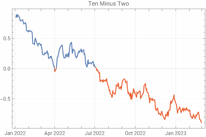
This plot shows the history of yield curve inversion using the ten year rate minus the two year rate as the criterion for yield curve inversion. When the ten minus two is zero or less, the difference is red on the plot and the yield curve is inverted. The yield curve inversion appears to be worsening by the ten-minus-two measure.
In[]:=
DateListPlotTranspose[{ycurves[[All,1]],#11[[2]]-#7[[2]]&@@@ycurves[[All,2]]}],
Out[]=
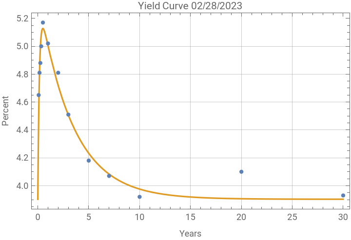
Here is the fit to the latest curve in the data. The last two points at 20 and 30 years maturity generally do not fit the model so they are dropped for the fit over the rest of this data analysis.
In[]:=
yModel=r0+(r-r0)(1-Exp[-at])UnitStep[t]Exp[-ct];nlm=NonlinearModelFit[Take[ycurves[[-1]][[2]],11],yModel,{r0,r,a,c},t];nlm["BestFitParameters"]ShowPlotnlm[t],{t,0,30},,ListPlot[Tooltip[#,#]&/@ycurves[[-1]][[2]]]
Out[]=
{r03.90277,r5.39547,a6.16142,c0.30181}
Out[]=
This function will be used to fit the data and output the fit as an Association for each curve.
In[]:=
yModelFn[t_,{r0_,r_,a_,c_}]:=r0+(1-)(r-r0)UnitStep[t];Clear[modelCurve];modelCurve[data_]:=Module[{nlm,data1},data1=Select[Take[data,11],#[[2]]=!=Missing[]&];nlm=NonlinearModelFit[data1,yModelFn[t,{r0,r,Abs[a],Abs[c]}],{{r0,data1[[1]][[2]]/2},{r,2data1[[-1]][[2]]},a,c},t];Association[#1->Abs[#2]&@@@nlm["BestFitParameters"]]];
-ct
-at
Fit all the curves in the dataset.
In[]:=
alist={};Do[ya=Quiet@modelCurve[ycurves[[i]][[2]]];AppendTo[alist,Join[Association["date"->ycurves[[i]][[1]]],ya,Association["yieldCurve"->ycurves[[i]][[2]]]]],{i,Length[ycurves]}]
In[]:=
Length@alist
Out[]=
288
The model was not appropriate for all the yield curves for the year. Only the fits where 0.1 < a < 30 are selected.
In[]:=
alist1=Select[alist,0.1<#[a]<30&];Length@alist1
Out[]=
267
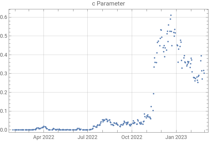
Here are the fits to the c-parameter, recall that when this parameter moves toward zero the yield curve is normalizing in shape. The selection criterion for alist1 shows curves before July with c near 0, which would be non-inverted curves. The market response to the FOMC action became more dramatic in November 2022. More recently the c-parameter appears to be decreasing.
In[]:=
cdata={#["date"],#[c]}&/@alist1;DateListPlotTooltip[#,#]&/@cdata,
Out[]=
So far the bond market has been determining the shape of the yield curve with the Fed only controlling the starting rate. There has not been an intervention to change the shape of the yield curve. Fed officials have offered macroeconomic explanations for yield curve inversions:
https://www.stlouisfed.org/on-the-economy/2018/september/why-yield-curve-invert-recession.
But these explanations don’t address the argument that I should buy short term Treasuries at a much higher yield rather than overpay for longer term Treasuries, because for the last two decades the Fed inflation projections have been mostly wrong and short term Treasuries have lower volatility and greater liquidity, without long term rate risk. I can always buy the longer term notes when the yield curve is more favorable.
https://www.stlouisfed.org/on-the-economy/2018/september/why-yield-curve-invert-recession.
But these explanations don’t address the argument that I should buy short term Treasuries at a much higher yield rather than overpay for longer term Treasuries, because for the last two decades the Fed inflation projections have been mostly wrong and short term Treasuries have lower volatility and greater liquidity, without long term rate risk. I can always buy the longer term notes when the yield curve is more favorable.
Microeconomics may better explain the yield curve shape. There are only 25 primary dealers participating, who make most of the bids, in Treasury auctions; their main clients are very large purchasers, including foreign governments, which are more interested in relative currency values than U.S. inflation. The Treasury decides the amount of each maturity to offer for sale before the auction, and it has continued to favor short maturities, despite the fact that the Fed has been pushing short term rates dramatically higher to the point where the debt limit will be exceeded early because of the high rates. The Treasury appears to be speculating that the FOMC will again lower the overnight rate to be less than the inflation rate. There likely is a significant supply-demand mismatch for both short term bills and longer term Treasury notes and bonds based on the size of the Treasury offerings for each maturity.
The question is whether the yModel can track the change in the yield curve shape as the yield curve normalizes. Using the yModel, the c-parameter should approach zero, when the yield curve has a shape similar to a scaled and range shifted exponential distribution. The following looks at the change of the c-parameter, selecting points starting on 15 Dec 2022; the highest point was on 21 Dec 2022. An exponential decay is chosen so that the c-parameter will stay above zero. The plot below shows a projection of a uniform decline of the data since December.
In[]:=
cdata1={AbsoluteTime[#1],#2}&@@@Select[cdata,#[[1]]>DateObject[{2022,12,14},"Day"]&];lm=LinearModelFit[{#1,Log[#2]}&@@@cdata1,t,t];bands[t_]=lm["SinglePredictionBands",ConfidenceLevel->0.95];p1=Plot[{Exp[lm[t]],Exp[bands[t]]},{t,AbsoluteTime[{2022,12,14}],AbsoluteTime[{2024}]}];ShowDateListPlotcdata1,,p1,
However, there is no reason to believe that the market should change the yield curve with a uniform decline in the c-parameter. The log plot below shows the data split by month, as there are monthly updates on the economy and inflation. The direction in February is not clear.
The monthly projections are less hopeful, but probably offer a more realistic way to track the data.
The a-parameter is the parameter for the implicit exponential distribution underlying the model. The fits where it is between 0.5 and 1.0 have a more normal appearance. It has been declining sharply recently.
The r0 and r-parameters do not change the shape of the yield curve, but they change its location and scaling on the y-axis of the plot. The r0-parameter should follow the FOMC overnight rate. The market appears to wait for the FOMC to act, rather than anticipating its action. The r-parameter, which is the maximal rate for the implied exponential distribution shape function, rose more rapidly when the FOMC began its operation. The interest rate spread appears to be stabilizing in the neighborhood of 1.5% suggesting that, if the FOMC controls inflation at 2% and sticks to its projected 2.5% overnight rate, the long maturity rate should end up near 4%.
Here is the point in time of the peak. The peaks before July 2022 were far enough out on the yield curve that they probably do not indicate full yield curve inversion, but they may add some information about how an inversion evolves. Recently the location of the peak has been moving further out in time; this should also be a measure of lessening inversion.
The peak rate of the function is rising, its future behavior should be interesting. It probably won’t decrease until the FOMC lowers rates.
This notebook is self-contained so it can be run each market day to follow the data. The Treasury generally updates the yield curve data at about 4:15 PM Eastern Time.