This notebook uses the NDSolve command to solve the differential equations that govern the motion of a Roberts’ linkage. The code solves the equations in three parts, since the equations have three different limit ranges. The animation shows the linkage moving from a starting position to a final position, and it can be used to visualize the motion of the linkage.
Type 1 Robert Linkage Rev D
Type 1 Robert Linkage Rev D
Parameters
Parameters
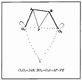
Figure1.Type1RobertLinkage,reference[1]
In[]:=
l=6;(*lengthA=lengthAB=length=l;length=2l*)
O
1
BO
2
O
1
O
2
Kinematic Analysis
Kinematic Analysis
Displacement Equations
Displacement Equations
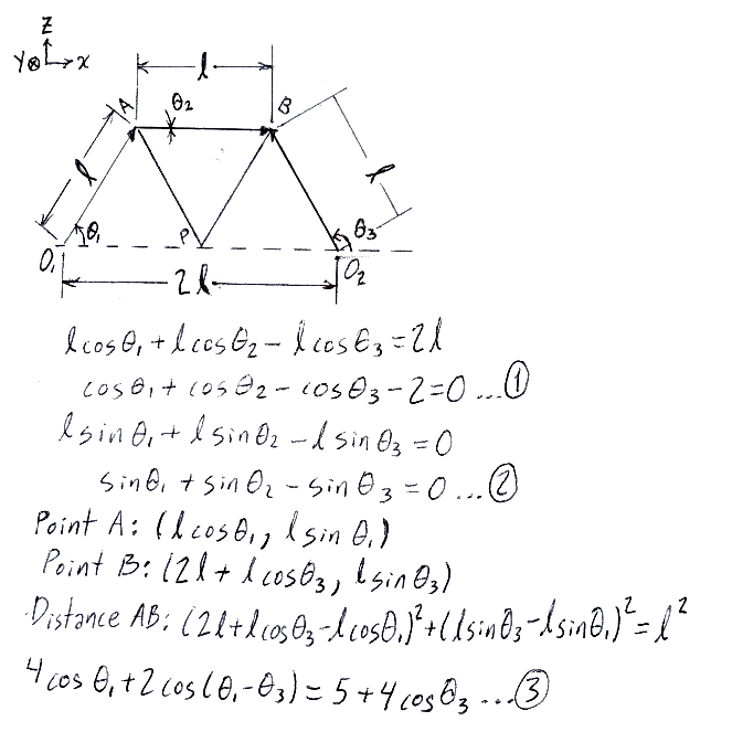
The displacement equations are obtained analyzing the mechanism geometryFigure 2. Equations 1 & 2 describe the x and z axis displacements, and Equation 3 is a geometric restriction for segment AB.
In[]:=
Clear[θ1,θ2,θ3];ξ=Cos[θ1[t]]+Cos[θ2[t]]-Cos[θ3[t]]-2==0;(*Eq.1alongxaxis*)ψ=Sin[θ1[t]]+Sin[θ2[t]]-Sin[θ3[t]]==0;(*Eq.2alongzaxis*)ρ=4Cos[θ1]+2Cos[θ1-θ3]5+4Cos[θ3];(*Eq.3isaconstraint:lengthAB=l*)
Velocity Equations
Velocity Equations
Clear[θ1,θ2,θ3];Dt[{ξ,ψ},t](*Derivingthedisplacementequationstoobtainasystemofdifferentialequationsthatarealsothevelocityequations*)
Out[]=
{-Sin[θ1[t]][t]-Sin[θ2[t]][t]+Sin[θ3[t]][t]0,Cos[θ1[t]][t]+Cos[θ2[t]][t]-Cos[θ3[t]][t]0}
′
θ1
′
θ2
′
θ3
′
θ1
′
θ2
′
θ3
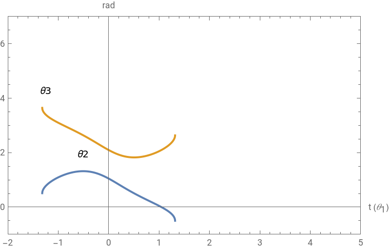
Solving for the unknown variables θ2 & θ3 (Part 3 of the Animation)
Solving for the unknown variables θ2 & θ3 (Part 3 of the Animation)
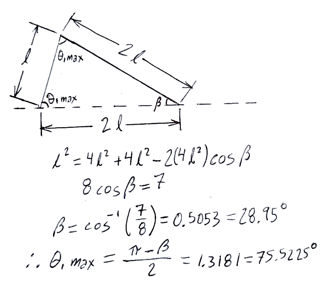
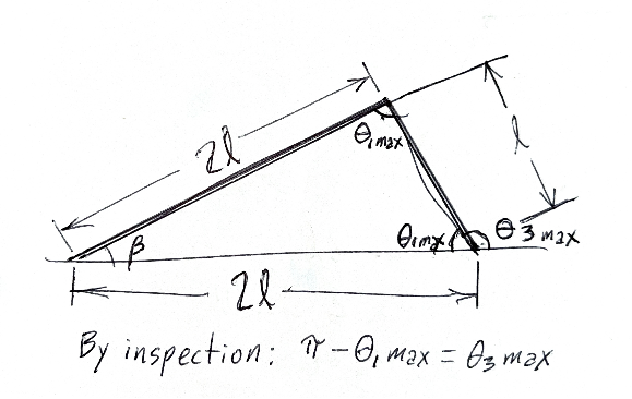
The entry angle, , is taken as a known input ( = t), and the input angular velocity is taken as = 1 rad/s. For more details, see reference [2].To obtain the range of the independent variable , from to , the cosine law is applied to the mechanism when the angle θ1 reaches its maximum value.This occurs when links AB and B are aligned, so the maximum distance between A and B through is 2l. Note that distance between and is also 2l, so points A, B and form an isosceles triangle at this instant.Figure 3. Determination of the value of the range, for the independent variable
θ
1
θ
1
′
θ
1
t
t
min
t
max
O
2
O
2
O
1
O
2
O
2
t
min
θ
1
In[]:=
mx1=1.3181;(*forrange*)
t
min
θ
1
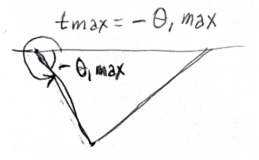
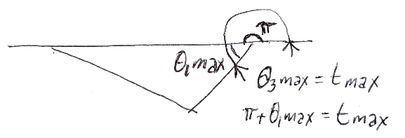
The maximum value, , of the independent variable range is simply Figure 4. Horizontal reflection of Figure 3 to determine the maximum value of the range, , for the independent variable .
t
max
-=-mx1
θ
1max
t
max
θ
1
In[]:=
s1=NDSolve-Sin[t]-Sin[θ2[t]][t]+Sin[θ3[t]][t]0,Cos[t]+Cos[θ2[t]][t]-Cos[θ3[t]][t]0,θ2[0]==,θ3[0]==,{θ2,θ3},{t,mx1,-mx1}(*SolvingtheODEsforθ1astheindependentvariable.Notethatθ1[t]isreplacedbytand[t]by1intheODEsorvelocityequations*)
′
θ2
′
θ3
′
θ2
′
θ3
π
3
2π
3
′
θ1
Out[]=
θ2InterpolatingFunction,θ3InterpolatingFunction


In[]:=
G3=Plot[Evaluate[{θ2[t],θ3[t]}/.s1],{t,mx1,-mx1},PlotLabelsPlaced[{"θ2","θ3"},Above],FrameTrue,AxesLabel{"t ()","rad"},Axes->True,AxesOrigin{0,0},PlotRange{{-2,5},{-1,7}},ImageSize->400](*plottingthesolutions*)
θ
1
Out[]=
Solving for the unknown variables θ1 & θ2 (Parts 1 and 2 of the Animation)
Solving for the unknown variables & (Parts 1 and 2 of the Animation)
θ
1
θ
2
In[]:=
Clear[θ1,θ2,t]
To complete the movement cycle, we take as the entry angle and the input angular velocity as = 1 rad/s. The minimum value of the independent variable range, , can be obtained by inspecting the figure below, which is the vertical reflection of Figure 3.Figure 5. Determination of the value of the range, for the independent variable
θ
3
′
θ
3
t
min
t
min
θ
3
In[]:=
mx2=π-mx1;(*for*)
t
min
θ
3
The maximum value of the independent variable range, , is simply Figure 6. Horizontal reflection of Figure 5 to determine the maximum value of the range, , for the independent value
t
max
π+=π+mx1
θ
1max
t
max
θ
3
In[]:=
mx3=π+mx1;(*for*)
t
max
θ
3
In[]:=
s2=NDSolve-Sin[θ1[t]][t]-Sin[θ2[t]][t]+Sin[t]0,Cos[θ1[t]][t]+Cos[θ2[t]][t]-Cos[t]0,θ1[π]==,θ2[π]==,{θ1,θ2},{t,mx2,mx3}(*SolvingtheODEsforθ3astheindependentvariable.Notethatθ3[t]isreplacedbytand[t]by1intheODEsorvelocityequations*)
′
θ1
′
θ2
′
θ1
′
θ2
π
3
5π
3
′
θ3
Out[]=
θ1InterpolatingFunction,θ2InterpolatingFunction


Animation
Animation
Animation Parameters
Animation Parameters
References
References
[1] RIUTORT, Kevin T. Applied design and implementation of straight-line mechanisms. 1996. Thesis Doctoral. Virginia Tech
[2] PAUL, B.; KRAJCINOVIC, D. Computer analysis of machines with planar motion: Part 1—Kinematics.
[2] PAUL, B.; KRAJCINOVIC, D. Computer analysis of machines with planar motion: Part 1—Kinematics.
CITE THIS NOTEBOOK
CITE THIS NOTEBOOK
Animating the dynamics of Roberts' linkage with numerical solutions of differential equations
by David Balandra
Wolfram Community, STAFF PICKS, July 2, 2023
https://community.wolfram.com/groups/-/m/t/2949486
by David Balandra
Wolfram Community, STAFF PICKS, July 2, 2023
https://community.wolfram.com/groups/-/m/t/2949486