We consider the higher order corrections to geodesic ball volumes on Riemannian manifolds and compute an assumed form of the higher order corrections to the Einstein field equations. The form of these corrections is highly undetermined. As a potential method of resolving this indeterminacy, we note an analogy that exists between the derivation of the Einstein field equations in the context of Wolfram models and the derivation of hydrodynamic equations from discrete molecular dynamics. In particular, we note that one might be able to use relativistic Burnett and relativistic super-Burnett equations to find explicit values to constrain the undetermined values in the higher order corrections to the Einstein field equations in the context of Wolfram models.
Introduction
Introduction
Where physics subfields meet - when there is only a hint of an underlying relationship - that is where the most exciting research can happen. With the development of Wolfram models and the parallel development of our understanding of what information they can convey (and how that relates to conventional physics) we are presented with many opportunities to extend our understanding.
The crux of the Wolfram physics project is to relate the discretuum to the continuum - a task that is both notoriously difficult and has exceptional promise. As physicists, we acknowledge the immense amount of time, effort and resources that have gone into finding a so-called Theory of Everything - some theory that might give a coherent description of physics at all scales; quantum and cosmological. While it is impossible to know whether the Wolfram physics project will take us all the way there, we would be foolish to sit idly by as others do all the ‘cool’ stuff. It is a part of the great pleasure of finding things out.
Einstein’s field equations (EFE’s) were first published in 1915 and are a representation of the fundamental relationship between the geometry of spacetime and the bodies that exist within it. The equations are represented by a tensor equation of the form
R
μν
1
2
g
μν
g
μν
T
μν
(
1
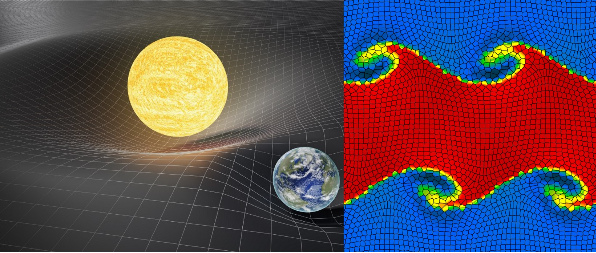
)where is the Ricci tensor, is the Ricci scalar, is the cosmological constant and is the energy-momentum tensor. The equation has remained unchanged for over a century and one should expect that finding corrections to these equations would be a challenge. There is, however, a potential method for finding higher order corrections. As Gorard found in his analysis of the relations between the Wolfram model of physics and general relativity [1], one may derive the EFE’s in the standard form (in the context of Wolfram models) by making use of geodesic ball volumes in the causal network of a hypergraph (this is a gross abbreviation of the process, but the method will be made clearer soon). In this essay, we discuss an extension of Gorard’s analysis and, in doing so, propose a method of finding an (indeterminate) form of the higher order corrections to the EFE’s.Of interest is how Gorard’s derivation is analogous to that of the derivation of the Navier-Stokes equations using the Chapman-Enskog method in the context of hydrodynamics. We conjecture that the indeterminate forms of the corrections obtained for the EFE’s may be determined by solving appropriate Burnett and super-Burnett equations.Below: A classic visualisation of general relativity (left) and results from a hydrodynamic simulation of the AREPO Code [6][7].
R
μν
R
Λ
T
μν
Higher Order Corrections to Geodesic Ball Volumes
Higher Order Corrections to Geodesic Ball Volumes
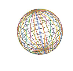
A geodesic describes the shortest path between two points on a manifold. There are various ways to visualise these but there is a particularly nice Wolfram repository function for these purposes. Most people are familiar with the geodesics on the surface of a sphere in 3-dimensional Euclidean space. The following code can be used for visualisation purposes [8].
(*UseResourceFunction["Geodesic"]toaccessthegeodesicrepositoryfunction*)sphere[a_][u_,v_]:={aCos[v]Cos[u],aCos[v]Sin[u],aSin[v]}ge=ResourceFunction["Geodesic"][sphere[1][u,v],{u,v},t,{0,0},θ]sg=Flatten[(NDSolve[#1,{u,v},{t,0,4}]&)/@Table[ge,{θ,(2π)/30,2π,(2π)/30}],1];sphere[1][u[t],v[t]]/.sg[[1]]/.t.1Show[{Graphics3D[Table[Line[Append[#,First[#]]&[sphere[1][u[t],v[t]]/.sg]],{t,0,3,1/5}],BoxedFalse],ParametricPlot3D[Evaluate[sphere[1][u[t],v[t]]/.sg],{t,0,π},BoxedFalse]}]
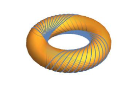
Which produces:A geodesic volume taken on the sphere (assuming we take the surface of the sphere to be some Riemannian manifold) is a 2-dimensional ‘bent’ disc. To see this, start from the upper pole and the move down until you hit a ‘latitudinal line’ - the enclosed area is a 2-dimensional ‘volume’.However, intuition begins to fail for less obvious structures. Consider a torus. What do its geodesics look like? We can visualise these again using the same repository function [8].
torus[a_,b_,c_][u_,v_]:={(a+bCos[v])Cos[u],(a+bCos[v])Sin[u],cSin[v]}ResourceFunction["Geodesic"][torus[3,1,1][u,v],{u,v},t,{2,3},θ]Show[ParametricPlot3D[Evaluate[torus[3,1,1][u[t],v[t]]/.NDSolve[ResourceFunction["Geodesic"][torus[3,1,1][u,v],{u,v},t,{π,π},.5],{u,v},{t,0,150}]],{t,0,150},BoxedFalse,AxesFalse],ParametricPlot3D[Evaluate[torus[3,1,1][u,v]],{u,0,2π},{v,0,2π},PlotStyleOpacity[.7],MeshFalse]]
O(
6
r
M
n
r>0
exp
m
r
M
m
V
m
exp
m
τ(R)=(Ricciscalar);||R=(NormofRiemanntensor);||ρ(R)=(NormofRiccitensor);ΔR=R=τ(R)(LaplacianofRicciscalar);and=2;
n
∑
i=1
R
ii
2
||
n
∑
i,j,k,l=1
2
R
ijkl
2
||
n
∑
i,j=0
2
R
ij
2
∇
n
∑
i=1
2
∇
ii
α
n
n
Γ
1
2
-1
Γ
n
2
the higher order corrections to the volume of an -dimensional geodesic ball are
n
V
m
α
n
n
r
n
τ(R)
6(n+2)
2
r
1
360(n+2)(n+4)
2
||
2
||
2
τ(R)
4
r
6
r
(
2
)As an aside, in -dimensional Euclidean space (r)=.What we now have are the higher order corrections to a geodesic ball on an arbitrary Riemannian manifold. Our primary goal, then, is to extend the analogy proposed by Gorard in [1] to higher order in . Geodesic balls can be taken in the discrete case by considering discrete steps of some characteristic length (conventionally one edge) on a hypergraph or causal network. To be more precise, a geodesic on a hypergraph between vertices and is the solution(s) to the shortest path problem. The discretization process of geometric objects and properties is described more completely in [1].
n
V
m
α
n
n
r
n
r
A
B
Derivation of the Form of the Higher Order Corrections
Derivation of the Form of the Higher Order Corrections
Consider an n-dimensional analytic Riemannian manifold, , and let be small enough so that is defined on a ball of radius in the tangent space . Then the ratio of the volume of a geodesic ball of radius in the manifold to the volume of a geodesic ball of the same radius in Euclidean space is
M
r>0
exp
m
r
M
m
r
V
m
V
E
τ(R)
6(n+2)
2
r
1
360(n+2)(n+4)
2
||
2
||
2
τ(R)
4
r
6
r
(
3
)While this relation might be sufficient when considering space alone, we must consider the spacetime form of this relation. To that end, Gray showed that the metric could be expanded to be of the form
g
pq
δ
pq
1
3
R
ipjq
i
x
j
x
1
6
∇
i
R
jpkq
i
x
j
x
k
x
1
120
2
∇
ij
R
kplq
16
3
R
ipjs
R
kqls
i
x
j
x
k
x
l
x
5
x
(
4
)where ∇ is the Riemannian connection and we use the convention that the Ricci scalar curvature is the contraction of the Ricci curvature tensor which is, itself, a contraction of the Riemann tensor in the first and third indices. That is
R=;and=.
ab
g
R
ab
R
ab
c
R
acb
Gray finds the higher order form of this procedure whose lower order terms agree with those found by Gorard. We can thus define the manifold’s volume element in terms of the standard Euclidean volume element (making use of the Einstein summation convention to neaten the results) by
dμ
g
1
6
R
ij
x
i
x
j
1
12
∇
i
R
jk
x
i
x
j
x
k
1
24
3
5
2
∇
ij
R
kl
1
3
R
ij
R
kl
2
15
R
iajb
R
kalb
x
i
x
j
x
k
x
l
5
||
dμ
E
(
5
)which leads to [2]:
det()=1--+-+-+O(||x).
g
ij
1
3
R
ij
x
i
x
j
1
6
∇
i
R
jk
x
i
x
j
x
k
1
24
6
5
2
∇
ij
R
kl
4
3
R
ij
R
kl
4
15
R
iajb
R
kalb
x
i
x
j
x
k
x
l
5
||
(
6
)Now, introducing the conventional Einstein-Hilbert action [3]:
S
EH
1
16πG
-g
4
1
16πG
-1--+-+-+O(||x)
1
3
R
ij
x
i
x
j
1
6
∇
i
R
jk
x
i
x
j
x
k
1
24
6
5
2
∇
ij
R
kl
4
3
R
ij
R
kl
4
15
R
iajb
R
kalb
x
i
x
j
x
k
x
l
5
||
4
(
7
)where and is the gravitational constant (which, along with the speed of light in a vacuum , we now set to be unity). Then our task is to extremize (as this is the general procedure for producing the EFE’s in a vacuum). This is quite challenging, and I was unable to minimize this during the last few days of the Wolfram Summer School.
At this point, it would not make sense to end the derivation abruptly. Rather, I will make a rather flimsy assumption and will proceed naturally thereafter - the main point being to outline the process one would go through to achieve the desired results.
Under the variation such that as , if we assume that the expansion of the metric behaves in approximately the same way as the unexpanded metric (this is the aforementioned flimsy assumption - it is almost certainly wrong) then with some tensor mathematics and several identities one can find [3]:
g=det()
g
ab
G
c
S
EH
At this point, it would not make sense to end the derivation abruptly. Rather, I will make a rather flimsy assumption and will proceed naturally thereafter - the main point being to outline the process one would go through to achieve the desired results.
Under the variation
gg+δg
δg0
||x||0
δRδRδ
-g
=-μκ
g
λν
g
g
κλ
R
μν
-g
+1
2
-g
μν
g
g
μν
(
8
)such that
This equation is based on a weak assumption made in deriving eq. 8. Nevertheless, the only significant challenge that one might expect that was not addressed here was the extremisation of the expanded metric. This would be the obvious place to start in a more accurate derivation of the corrections to the EFE’s. While eq. 13 is quite devoid of things that might allow one to have an intuition of what is going on, we do have potential ideas for resolving this.
Proposed Method for Resolving Indeterminacy
Proposed Method for Resolving Indeterminacy
A brief look at the analogy
A brief look at the analogy
We consider the case of a hypergraph and then move to the case of a causal graph. In all examples we run the same initialisation code:
Consider some hypergraph that meets the criterion specified (causal invariance, asymptotic dimensional stability). A good example of such a hypergraph that appears to have a good correspondence with a 2-dimensional Riemannian manifold is WM7714. The code shown will produce the image shown if the second ‘Automatic’ is changed to ‘2500’.
Noticing that geodesic balls in a causal graph give a sort of distribution function and, therefore, recognising the link between the corrections to geodesic ball volumes in arbitrary Riemannian manifolds, distribution functions and the relativistic hydrodynamic equations, one can - at the very least - constrain the undetermined correction values in the higher order EFE' s by recognising analogous structures. This has the potential to influence the way we understand spacetime near singularities (such as black holes).
In summary, we know the corrections to the volumes of geodesic ball volumes from [2]. We have a means of calculating the EFE' s in the discrete hypergraph case (with certain constraints) from [1]. We have the form of the indeterminate higher order corrections to the EFE' s (this work). Finally, we have a means of removing the determinacy by using the Chapman - Enskog method to constrain the undetermined values (by analogy, as noted in [1]). As a result of constraining the values in the higher order EFE' s, one can obtain (to an as yet unknown determinacy) the higher order EFE' s.
In summary, we know the corrections to the volumes of geodesic ball volumes from [2]. We have a means of calculating the EFE' s in the discrete hypergraph case (with certain constraints) from [1]. We have the form of the indeterminate higher order corrections to the EFE' s (this work). Finally, we have a means of removing the determinacy by using the Chapman - Enskog method to constrain the undetermined values (by analogy, as noted in [1]). As a result of constraining the values in the higher order EFE' s, one can obtain (to an as yet unknown determinacy) the higher order EFE' s.
A Brief Look at the Complexities to be Overcome
A Brief Look at the Complexities to be Overcome
Then the general equation of transfer is:
and
What we have seen in this section is, once again, a very brief description of the proposed method for resolving the indefiniteness to the EFE's. Despite the seemingly high density of equations, the reader can be assured that this is a gross abridgement of the process. Once again, it is emphasized that this is a non-relativistic demonstration of the principle. A relativistic formulation will certainly have its own subtleties, but we shall not address them here.
Finally, notice that we have been discussing continuous hydrodynamic equations in the context of Maxwellian/Hard-sphere discrete molecules. The derivation of continuous equations from a fundamentally discrete system are what give weight to the link between the derivation of the EFE’s in Wolfram models and the derivation of hydrodynamic equations from a discrete system.
Conclusions
Conclusions
We have briefly investigated the higher order corrections to the EFE’s. We did not successfully extremize the altered form of the Einstein-Hilbert action, but proceeded with our discussion, regardless of this, to demonstrate the idea as opposed to an exact result. We thus found an undetermined form of the higher order corrections to the EFE’s and proposed that a Chapman-Enskog expansion of the relativistic Boltzmann equation might allow us to put restrictions on the undetermined values in the higher order EFE’s by recognising analogous structures. We also gave a very short and incomplete explanation of the idea (a full explanation would require more than 50 pages) used in the Chapman-Enskog expansion.
Future work is needed to properly extremize the Einstein-Hilbert action as well as to deal with the challenging process of finding the constraints through the Chapman-Enskog method - but these results have the potential to alter how physicists interpret spacetime near singularities. The Mathematica-compatible tensor package xAct [5] may make the extremization process trivial to an individual familiar with the software. There are papers on the relativistic Burnett equations and this must necessarily be consulted in order to perform a full analysis of the EFE’s. It has also been suggested (in a very informal sense) that there may also be links to dark matter that can be explored from these corrections.
It is my hope that I might develop this work to completion (if such a thing as ‘completion’ can be said to exist in physics) in the near future.
Acknowledgment
Acknowledgment
Mentor: Jonathan Gorard
In all my ‘playing’ with Wolfram models I made use of so many of the Wolfram resource functions written by Max Piskunov and I owe him a debt for writing functions that are both powerful and easy to use.
I would like to thank Stephen Wolfram for bringing together such an interesting group of students to work on novel ideas together - without such environments the many fields of science would stagnate. His will to power is both impressive and infectious.
I would be wrong in failing to mention Jesse Friedman, who was able to resolve countless queries of both myself and the Summer School group at large. He is truly a phenomenal problem solver of all things Mathematica.
Finally, I am honoured to have worked under someone so brilliant as Jonathan Gorard. I am deeply indebted to him for his willingness to assist me at every step of the process of producing this project. Without question, none of my newfound insight would be possible without him. He also has a wonderfully keen sense of humour.
References
References
◼
[1] J. Gorard (2020). “Some Relativistic and Gravitational Properties of the Wolfram Model”. https://www.wolframcloud.com/obj/wolframphysics/Documents/
some-relativistic-and-gravitational-properties-of-the-wolfram-model.pdf
some-relativistic-and-gravitational-properties-of-the-wolfram-model.pdf
◼
[2] A. Gray (1974). “The volume of a small geodesic ball of a Riemannian manifold.” Michigan Math. J., Volume 20, Issue 4 (1974), 329-344. https://projecteuclid.org/euclid.mmj/1029001150
◼
[3] M. Nakahara (2003). “Geometry, Topology and Physics.” Second Edition. Pp 297-302.
◼
[4] A. Agrawal et al (2020). “Microscale Flow and Heat Transfer”. Springer Mechanical Engineering Series. Pp 125-188.
◼
[5] J. Gargcia et al (2020). http://www.xact.es/.
◼
[7] Taken from https://www.h-its.org/2014/10/28/arepo/
◼
[8] Wolfram Staff (original content by Alfred Gray). Code snippets taken and manipulated from https://resources.wolframcloud.com/FunctionRepository/resources/Geodesic