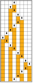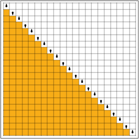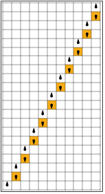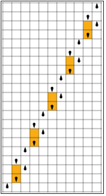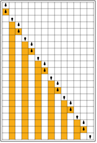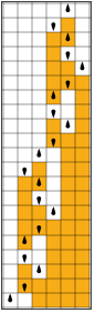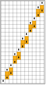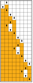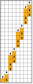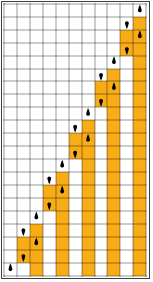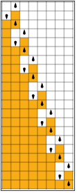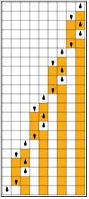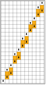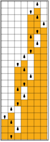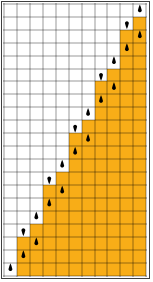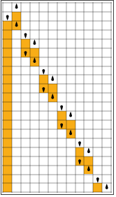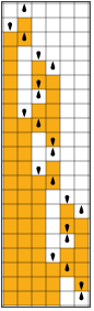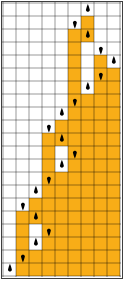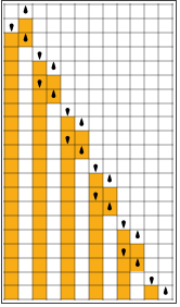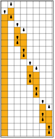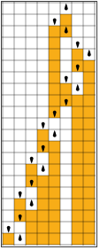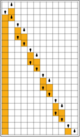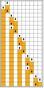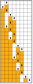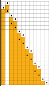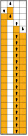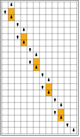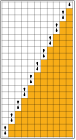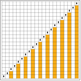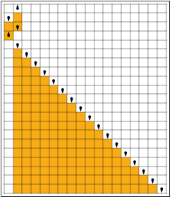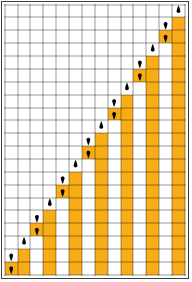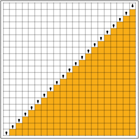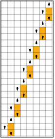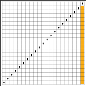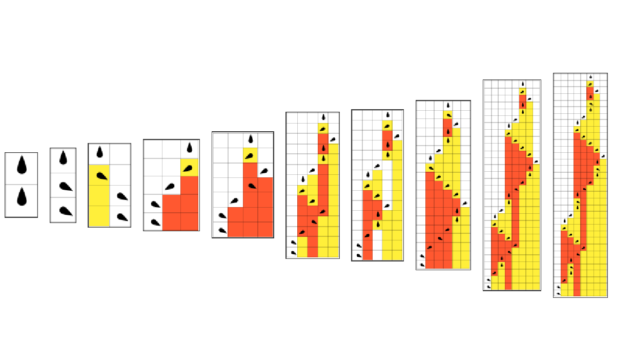
When we think of biological systems, all the time we don’t actually have a way of describing them, therefore lack an understanding of what’s going on underneath these systems as they undergo evolution. This project tries to ignore some of the constraints that we may encounter in biological systems namely “we don’t know what’s going on” and essentially think of biological organisms as computational systems with certain sets of rules they follow to develop. These rules are equivalent to the genotype of the organism and the result of executing them as its phenotype. We take a minimal model for biology that has this setup, Turing machines, and study their adaptive evolution.
​
The main idea is to have a Turing machine with configurations of n-colors, s-states, and a rule . We then run the machine for a number of steps, changing the rule each step to find a pattern that lives the longest.
​
This is an attempt to the famous busy beaver problem but with a different approach of trying to evolve busy beavers to find one the lives the longest.

A Minimal Model for Biological Evolution and Adaptive processes

A question one could potentially ask is how does biological evolution work or for that matter, why does it work? Here, we explore this question and more using a minimal model for biological evolution and some adaptive processes.

Introduction to The Model

Notes for this notebook

◼
  • 2-state, 2-color machines 4096 rules
  • ◼
  • s-state, k-color machines (2 s k)^(s k) rules
  • ◼
  • A single rule {state, color} -> {newState, newColor, direction}
  • ◼
  • List of rules {singlerule1, singlerule2, singlerule3, ..., }
  • For our project, we will focus on all the above.
    The 3-state, 3-color, using the above, we have rules totalling to:
    In[]:=
    (2×3×3)^(3×3)
    Out[]=
    198359290368

    Define halt state

    Let us consider a simple example of what we will be discussing in this project.
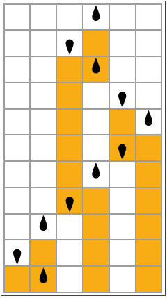
    Given the example rule below: (2 2) TM rule:
    In[]:=
    rule={{1,0}->{2,1,-1},{1,1}->{2,0,1},{2,1}->{1,0,-1},{2,0}->{1,1,1}};
    Here’s the evolution of a Turing machine based on the rule with only 10 steps.
    In[]:=
    RulePlot[TM[rule],{1,{{},0}},10,MeshAll,ImageSize120]
    Out[]=
    Now, let’s think about how we can evolve a system from a single point like the one below to a system like the one above without setting any explicit rule like we did above but mutating a certain rule, which in this project we call a null rule, then after a certain number of evolution steps we observe what happens.
    Let say we start from the single point below:
    In[]:=
    nullEvolution=TuringMachine[{{1,0}->{1,0,0}},{1,{{},0}},0];​​RulePlot[TM[#->{1,0,0}&/@Tuples[{Range[3],Range[0,2]}]],nullEvolution,ImageSize50]
    Out[]=
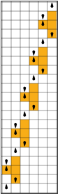
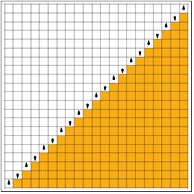
    The expected behaviour for a system with null rule, of course, is that it immediately dies out for a program like a cellular automata. But since we are going to use a different program; Turing machine, the expected behaviour is for this machine to run forever or up to a finite number that you have set the program to run without changing any state. So if we run the above machine again for some steps, the following should be expected.
    In[]:=
    testrule=#->{1,0,0}&/@Tuples[{Range[3],Range[0,2]}];​​nullEvolutionTenSteps=TuringMachine[testrule,{1,{{},0}},2];​​RulePlot[TM[testrule],nullEvolutionTenSteps,ImageSize50]
    Out[]=
    As you can see the system just keeps going without doing anything. This is good for us because we can use this realization to check the evolution of our system later on when we actually start doing changes to the state of the system or for our case; do random “point mutations” to the system.
    ​
    How will that work? Well, we will evolve the system by changing it, then detect the point the system starts repeating itself or gets stuck in an infinite loop. After we find where the system gets in a loop, we can then use that as a halt state so that whenever we get to that state, we halt the evolution of the system and make judgements(usually based on performance of the system) in regards to what we want to do to the system.
    We set the halt state to something like below; this is for the example. Later on we will see how to set for all the rest of the rule.
    In[]:=
    haltRule={1,0}->{1,0,0};
    If we look at the test rule below, we can see the halt state as the first rule.
    In[]:=
    testrule//Column
    Out[]=
    {1,0}{1,0,0}
    {1,1}{1,0,0}
    {1,2}{1,0,0}
    {2,0}{1,0,0}
    {2,1}{1,0,0}
    {2,2}{1,0,0}
    {3,0}{1,0,0}
    {3,1}{1,0,0}
    {3,2}{1,0,0}
    Let us plot the rules and see how it looks like:
    In[]:=
    RulePlot[TM[testrule],ImageSize->Large]
    Out[]=
    With this, whenever our system gets to the first state in the plot above, it halts its evolution.
    How can we make use of the halt state? In the following sections we perform random “point mutations” to our system and observe how it behaves. But first, let’s describe how the single point mutation model works below:

    How the single point mutations model works?

    Let’s dive deep to see the working of the simple model we are proposing. First, for a (2 2) TM, we have 2 * 2 = 4 cases in the rule: Note that a case is represented by {state, color} -> {newState, newColor, direction}. And to each case, we perform a single point mutations. This means we will have, for a single case in our rule, total = (state * color * number_of_directions) possible mutations defined from state, color and direction.
    ​
    For example, let’s consider the rule below as our original:
    In[]:=
    RulePlot[TM[rule],ImageSize300]
    Out[]=
    Now, for every case in the rule above, we get all possible mutation starting from index 1, 2, 3, ..., n changing only one point in the rule, where n is the number of cases in the rule. The above rule, (2 2) TM rule, will have a total of (state * color * number_of_directions) * number_of_cases = (2 * 2 * 3) * 4 = 48. Note: We subtract number_of_cases to remove duplicates of the original rule as it is not a mutation. So for this case we will have 48 - 4 = 44.
    In[]:=
    GetAllPossibilities[rule,{2,2}]//Length
    Out[]=
    44
    With this in mind we can plot, below, all possible mutations evolution:
    In[]:=
    PlotRulesEnumeration[rule,First/@GetAllPossibilities[rule,{2,2}],20,20,672113]
    Out[]=
    
    ,
    ,
    ,
    ,
    ,
    ,
    ,
    ,
    ,
    ,
    ,
    ,
    ,
    ,
    ,
    ,
    ,
    ,
    ,
    ,
    ,
    ,
    ,
    ,
    ,
    ,
    ,
    ,
    ,
    ,
    ,
    ,
    ,
    ,
    ,
    ,
    ,
    ,
    ,
    ,
    ,
    ,
    ,
    As you can see a single point mutation made to one case can affect the system significantly.
    Some of the rules go on forever, others have a lifetime that is less than the parent rule, and others have the same lifetime as the original rule. In the next sections, we will see how to perform random point mutation and selection of the rules that we care about from all these possibilities. Essentially, what we want is to ignore all the rules that lead to a lifetime less than the parent and those that go on forever but select only those that improve the lifetime or lead to the same lifetime as the parent.

    Turing Machine Random Point Mutations

    Previously, we saw how to get all possible mutations. Here, we will just get a random point and get all possibilities for the specific point. We refer to random point mutations here’s as picking a single case in a rule at random and changing one outcome in the case then adaptively evolving the system. To perform mutations, let us consider a 3-state, 3-color Turing machine, also refer to here as (3 3) TM. For a (3 3) TM consider a single case, i.e., picking {1, 1} -> {2, 1, 0} as a single random case, we have (3 * 3 * 3) = 27 possible mutations. Considering all all possibilities, we have 27 * 9 = 243(9 is the number of cases in the ( 3 3) TM). Later on we can demonstrate how other Turing machines can be changed and evolved.
    First, we want to make sure our null rule reflects our definition of halt state. Essentially, we want all the cases in our null rule to be halt states, that way the system halts immediately at the start of the evolution and before mutations.
    Let’s define our null rule:
    With a beginning of our evolution setup, let’s now do changes to our system and adaptively evolve it.

    Perform single point mutations on null rule

    Copy the nullRule:
    Get all 27 possibilities for the (3 3) TM null rule:
    Plot all 27 possible rules(3 for color change, 3 for state change and 3 for direction change): We are only showing the first 7 in the plot below.
    If you observe closely through the rules above, you will notice some changes compared to what we had initially in the nullRule. This suggests a change in the rule.
    We can visualize the evolution for the above rules:
    Clearly, nothing happens to the system. It seems to go on forever; not exactly what we want. Well, this is expected because the system hit the halt state immediately even after mutation. To see a change, we need to run it multiple times as we do changes to it.
    ​
    The above system only shows 3 evolution steps even though we run for 50 steps. What’s happening is that we detected that the system entered a halt state and stopped it’s evolution then determined how long it lived before it hit this state. The process of determining this is by performing fixed point to the system to only get the part that we are interested in, in this case, the life time of the system before halting. This is called fixed point but in this project we refer to it as lifetime of the machine. In the above case we only got a lifetime of 3 for both cases.
    From the above, even though the lifetime of the machines is larger than the origin, these are not considered as evolved systems because they immediately hit the halt state with the same head state as the origin. In the next section, we will see how to determine lifetime of a system through an evolution algorithm that adaptively evolves the system.

    Turing Machine Lifetime Selection

    I described here how the lifetime selection is done.
    First, confirm our null rule has not changed to test the new evolution.
    The goal, here, is to run as many Turing machines as possible to get the one that lives the longest lifetime. In each step, we will also keep track of all possible generations that our winner came from but only those that evolved more than the previous generations of the machines. At the end we expect a list of all the machines that made progress or were accepted to move on to the next generation. Below is a procedure we will follow;
    ◼
  • We perform random point mutation, done in the previous section, on the null rule to get all possibilities i.e state + color
  • ◼
  • Evolve all (state * color * 3) possibilities in parallel to get their life time and accumulate all their lifetime
  • ◼
  • Check for the machine that made a step in the process by comparing each of the possibilities’ lifetime against the previous machine.
  • ◼
  • If one machine is found with lifetime that is greater or equals to the previous machine, we accept it to move on to the next generation
  • ◼
  • If multiple are found, we pick one at random to move on to the next generation
  • ◼
  • Otherwise, we reject the machines and eliminate it from the evolution process
  • ◼
  • We repeat the steps above, keeping track of all accepted machines
  • ◼
  • We then filter out all the machines that made it
  • It turns out with this procedure, as we will see shortly, we can adaptively evolve to new patterns.
    To test this process, let’s run our algorithm to perform evolution for 500 steps and a cut off of 50; cut off is the maximum number of lifetime we want to have, i.e., if an evolution has a lifetime greater than cutoff, we consider it going forever. Here, we just set to a minimum number as possible for demonstration. You can play around with larger values. Note: SeedValue changes the state of the random generator algorithm.
    As you can see above, a simple form emerges, then as the adaptive process goes on, the system starts to develop large forms. Its interesting to just think about it because you can imagine what sort of patterns we might get if we ran the system for a long but finite number of steps or even infinite time steps.
    ​
    You might wonder how much time did a system in the above pattern take to evolve to the next generation. The following plot shows a trace of the whole adaptive evolution process.
    ​
    To see what’s going on, let’s make a plot for the maximum lifetime achieved so far against the total number of mutation steps made. We will include rejected just to see all the activities happening in our evolutionary process.
    The red dots in the plot above show those machines that never make it to the next step while the blue line represents the trajectory the evolution process takes at every step. It’s clear from the above plot that as much as we are evolving and seeing emergence of larger patterns, we are still bias to quite a lot of systems because out of the many red dots you see, there could be systems that do well if more mutations were done to it. One of the things we will do is check how many of the red dots run forever and try to determine or predict whether they will halt. This is referred to computational irreducibility.

    Comparison to Other Turing machines

    2-state, 2-color Turing machine

    All possible rules for (2 2)TM:
    Set the null rule for (2 2)TM:
    Evolution plot:
    ◼
  • Mutation happening one at a time.
  • 3-state, 2-color Turing machine

    All possible rules for (3 2)TM:
    Set the null rule for (3 2)TM:
    Evolution plot:
    ◼
  • Mutation happening one at a time.
  • 4-state, 3-color Turing machine

    All possible rules for (4 3)TM:
    Set the null rule for (4 3)TM:
    Evolution plot:
    ◼
  • Mutation happening one at a time.
  • Evolution growth for all Turing machines

    Let’s plot the evolution growth for all the machines we saw above and see how they compare in their growth with each evolving the same number of steps. Change steps from 2000 to a lower number for faster execution.
    From the above, it seems to suggests TMs with larger states starts to evolve much later in time. For example, TM (2 2) evolves fast at the beginning but stops almost immediately for the number of steps used here. And if you look at TM (4 3), evolution start much later. But the interesting fact about it is its evolution starts later than all other machines with less states.

    The Multiway Graph of All Possible Mutations Histories

    Let’s look at the process using multiway graph. The multiway graph will help us understand what’s actually going on in the evolution process, we can create a map of all relationship between previous generation of machines to the current. Here, we will focus only on (2 2) Turing machine but you can try them all out for yourself by changing the argument for {state, color} in the MultiwayGraph function.
    ​
    Please note that the results here are preliminary as we are picking a random point and mutating it by considering only one possibility. For example, this rule, {1, 1} -> {2, 1, 0}, for TM(2 2), has 12 possibilities, but we are only considering one of these possibilities. Also, the algorithm does not handle cases where the previous machine immediately hits a halt state, in which case they are the same.
    ​
    ​Update: The algorithm has been updated to handle the above(all possibilities).
    (2 2) Turing machine:
    Let’s start with our null rule as the root/parent node.
    Typically, a rule has as many children as the number of cases in the list of rules but considering the number of state and color, each child (case) in the list of rules spawns (state * color * 3)* (state * color) possible mutations which makes the possibilities grow as the number of state and color increase.
    We can see below all the possible mutations found from the parent rule:
    We can then run the above enumeration through a multiway graph to see clearly what is happening and how the relationship are created from a null rule or parent to all the children machines that make progress. The multiway graph below shows all the possible paths to take from the parent machine (parent machine being the null rule) to the last children machines. The graph displayed is for (2 2) Turing machine with single point mutation performed.
    The way the evolution is performed is:
    ◼
  • Take each child/case in the parent rule and enumerate the n = (state * color * 3)* (state * color) possible mutations for that child
  • ◼
  • Evolve each of the n possible mutations one at a time, checking the lifetime of the evolved rule against the parent life time
  • ◼
  • If the lifetime for the evolved mutation is greater or equals to the parent, we keep it, otherwise we reject
  • ◼
  • If the mutation lead to infinite lifetime, we reject it
  • ◼
  • Store all the lifetime that evolved to run them in a multiway graph
  • ◼
  • We do this as many times as possible. In our case, we use layers to run the evolution. The MaxLayers option below will determine how many times the evolution should run.
  • The next multiway graph shows all the mutations done on each machine child and the result of the child evolution after mutation. The result is selected as in lifetime selection above where we take those “children” that make progress. Here, we determine progress by comparing the evolution of a machine child to the parent machine, if child lifetime is greater than or equal to the parent, we move the child to the next generation.
    ​
    Let’s look at the parent tree on a multiway graph by running the above evolutionary algorithm to get all the evolutions that made it:
    ​
    Evaluating for 3 layers of the tree:
    In the previous evolution process, we have been taking machines whose evolution produced a lifetime of greater or equal to the parent machine they came from. That is evident with a lot of machine with same lifetime as the parent machine in the previous multiway graph. We can restrict the process so that we only allow machines that evolve with greater lifetime than the parent machine. Below, we can see a multiway graph with only those machines that made progress. The number is reduced and we do not have a lot of repetition as before.
    We can imagine going much deeper into the tree with more layers and only taking those machines with lifetime greater than the previous. Let’s see how that looks like below:

    Future Work

    ◼
  • Trying out different mutations strategy like sexual Reproduction for Turing machines and multiple point mutations.
  • ◼
  • Exhaustive search of the complete search space of all possible rules
  • ◼
  • Undecidability: In this project, we have been ignoring systems that go on forever with the assumptions that they may never terminate but we cannot be sure about that. My future work will consider those systems and try to predict ahead of time whether they will terminate or not.
  • ◼
  • Proof construction for telling whether a system that is undecidable will halt or never will.
  • Concluding Remarks

    The result found here seems to suggest that adaptive evolution can happen in a system provided the system changes. This is true as well for biological systems where the entire system depends on genes to evolve, and any edits to these genes can significantly affect the system’s evolution. The only real question is how should the changes/edits happen for better results? Because as far as evolution is concerned, good is not desirable.

    Acknowledgments

    I would like to thank my mentor Eric James Parfitt for guiding me through the project, Stephen Wolfram for the initial project idea and to all the Wolfram staff who helped organize the 2024 Wolfram Summer School.

    References

    ◼
  • Stephen Wolfram, A New Kind Of Science, Wolfram Media (2002). ISBN: 1-57955-008-8
  • ◼
  • Stephen Wolfram, Why Does Biological Evolution Work? A Minimal Model for Biological Evolution and Other Adaptive Processes, May 3, 2024
  • ◼
  • Geometry of Program Synthesis
  • ◼
  • Mutation-selection dynamics and error threshold in an evolutionary model for Turing Machines
  • ◼
  • Busy beaver
  • ◼
  • With Fifth Busy Beaver, Researchers Approach Computation's Limits
  • Cite This Notebook

    Adaptive evolution for Turing machines​
    by Brian A. Mboya​
    ​https://community.wolfram.com/groups/-/m/t/3209199