Krugman's Model of Increasing Returns and Monopolistic Competition

labor

cost function parameters

0.5

wages

MR, MC

dashed lines

check

number of firms

n =

1.00

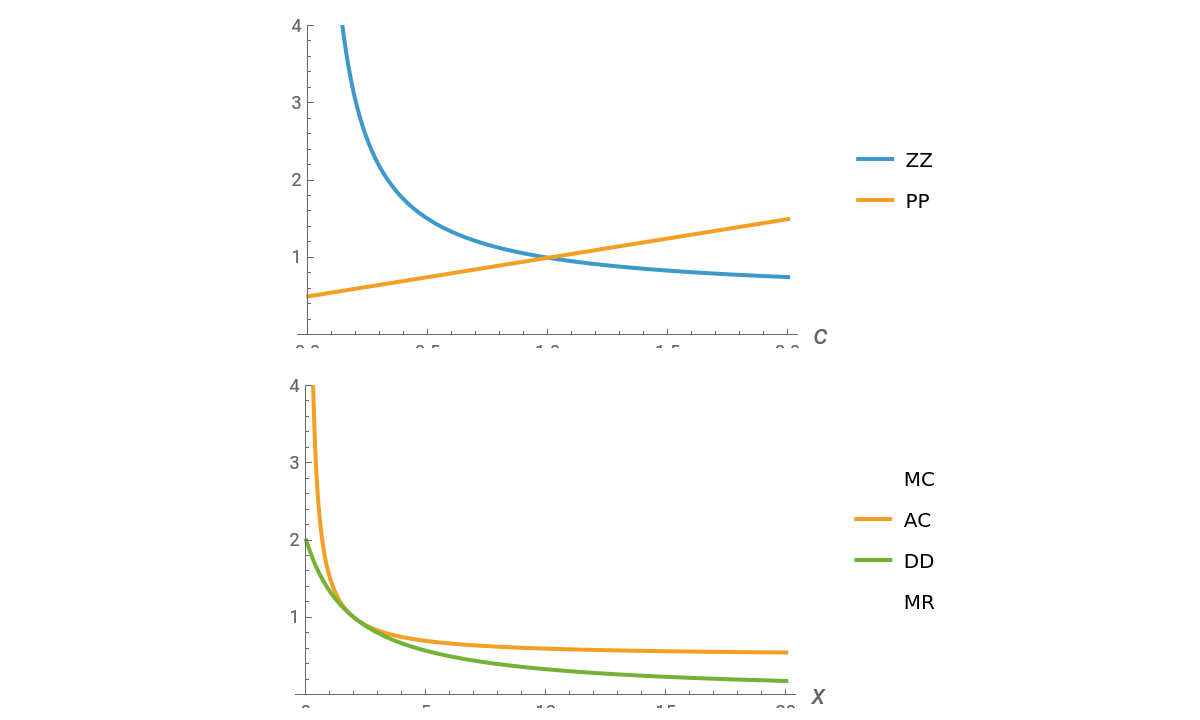
This Demonstration considers Krugman's model of increasing returns and monopolistic competition. Krugman's model can be applied to international trade or the economics of agglomerations. Originally, Krugman considered equilibrium in terms of the relationship between price

and consumption

(upper plot). This Demonstration adds the more familiar inverse demand representation (bottom plot), which shows the relationship between price

and the production quantity

. Notice that the typical output of a firm and the typical consumption by an individual have the following dependence:

x=cL

, where

is the whole population (total labor)—that is, the main parameter of the model.

All curve labels are constructed as follows:

for marginal revenues,

for marginal costs,

for average cost and

for demand (inverse).

and

are notations used by Krugman[1, pp. 474], where the first reflects

p/w=β+α/(Lc)

and the second shows

p/w=β(1-ϵ)/ϵ

derived from the Amoroso–Robinson formula. These two curves have no special interpretation in theory, but merely demonstrate the relation of

and

in the model. That is why it is instructive to bridge the model with a more conventional visualization of monopolistic competition.

Details

Krugman considered the inverse demand function in a general form

-1

v'(c)

and that

v(c)

should be chosen such that elasticity of demand

decreases with

. The usual requirements

v'(c)>0

v''(c)<0

also apply. To visualize the model, we take

v(c)=log(1+c)

, which provides the most tractable results:

1+c

where

μ=

-1

One may check that elasticity

ϵ=

1+c

is decreasing with

. Remember that

, where

is an exogenous population.

Increasing returns in the one-factor case

can be modeled as

l=α+βx

, which is the inverse production function.

To get the total costs function, we need the factor price

TC=wl=w(α+βx)

so average costs are:

AC=w

+β

In the monopolistic competition case, the following system should be resolved:

AC=DD∧AC'=DD'

Interestingly, while solving the system we may simultaneously obtain

Lα

and

μ=

w

Lβ



This solution shows how demand walks around the average costs curve while

changes (bottom plot). Notice that the number of firms in a growing market also increases, while individual consumption of each good decreases. This means growing diversity and volume of consumption for a representative consumer.

Unlike Krugman's original paper, we put

on the vertical axis of the upper plot instead of

p/w

, but as

is exogenous, this does not influence the exposition (we just let the upper plots depend on the

parameter).

This model may describe international trade or agglomeration effects because an increase of

corresponds to market extension. This simple model ignores transportation costs, but they may be incorporated as well, as Krugman shows in his later works.

References

[1] P. R. Krugman, "Increasing Returns, Monopolistic Competition, and International Trade," Journal of International Economics, 9(4), 1979 pp. 469–479. doi:10.1016/0022-1996(79)90017-5.

Permanent Citation

Timur Gareev

"Krugman's Model of Increasing Returns and Monopolistic Competition"
http://demonstrations.wolfram.com/KrugmansModelOfIncreasingReturnsAndMonopolisticCompetition/
Wolfram Demonstrations Project
Published: June 18, 2018