Wolfram Cloud Page

Dynamics is the branch of mechanics concerned with the motion of physical systems. It can be divided into two main areas: kinematics and kinetics. Kinematics studies three fundamental characteristics of motion (position, velocity, and acceleration) as functions of time. Kinetics, on the other hand, relates the motion of a system to its causes, such as the forces and moments acting on it. Our focus will be on deriving the equations of motion using three different but equivalent formulations: Newton’s approach, Lagrange’s approach, and Hamilton’s approach. While Newton’s approach uses vector forces and is well suited to simple dynamical systems, analytical mechanics employs scalar energy quantities through the Lagrangian and Hamiltonian formulations, making it more convenient for complex systems. Although these approaches differ in their mathematical formulations, they ultimately produce equivalent equations of motion for the same physical system. This project provides a simple introduction to these three formulations of mechanics and uses Wolfram Language to implement each formulation. The approaches are then applied independently to several conservative mechanical systems:

Mass-Spring System

Simple Pendulum

Atwood’s Machine

Projectile Motion

Gravitational Central Force Field

Spherical Pendulum

Double Pendulum

Formulations of the Equations of Motion

The equations of motion of a mechanical system can be derived through several equivalent formulations. In this section, three fundamental formulations for conservative systems are presented: Newtonian mechanics, represented by Newton’s second law; Lagrangian mechanics, represented by the Euler–Lagrange equations; and Hamiltonian mechanics, represented by Hamilton’s canonical equations. The same underlying dynamics is described through vector forces in Newtonian mechanics and scalar energy quantities in Lagrangian and Hamiltonian mechanics. Generalized coordinates and generalized velocities are used in Lagrangian mechanics, whereas generalized coordinates and conjugate momenta are used in Hamiltonian mechanics. These formulations are first presented mathematically and then implemented using Wolfram Language.

Newton’s Approach: Newton’s approach is based on relating the forces and moments acting on a system to its resulting motion. Since forces are vector quantities, they often need to be resolved into suitable components, typically with the aid of a free-body diagram. This formulation is direct and intuitive for simple dynamical systems but can become increasingly difficult for complex systems involving multiple bodies or constraints. The relation between the net force

ℱ

and the resulting motion is established by Newton’s second law, which states: “When observed from an inertial reference frame, the net force

ℱ

acting on a particle is equal to the time rate of change of its linear momentum.” Assuming a constant particle mass

and denoting its velocity by

, Newton’s second law is expressed as:

ℱ

(

)

Construct Newton’s equations of motion:

In[]:=

newtonEquations[ℱ_List,m_,a_List]:=Reverse/@Thread[ℱ==m*a]

Lagrange’s Approach:
Lagrange’s approach derives the equations of motion from the kinetic and potential energies of a system rather than from the forces acting on it. Since energy is a scalar quantity, this formulation avoids much of the vector analysis required by Newton’s method. It is particularly effective for complex dynamical systems, especially those involving multiple degrees of freedom or constraints. The Lagrangian is defined as:

ℒ(q,q̇,t)=(q,q̇,t)-(q,t).

(

)

Here,

(q,q̇,t)

is the kinetic energy,

(q,t)

is the potential energy,

q=(

,...,

)

is the generalized-coordinate vector, and

q̇=dq/dt=(

q̇

,...,

q̇

)

is the corresponding generalized-velocity vector. Once the Lagrangian has been constructed, the

equations of motion associated with the

generalized coordinates are obtained from the Euler–Lagrange equations:

∂ℒ

∂

q̇

∂ℒ

∂

,i=1,2,...,n.

(

)

Here,

∂ℒ/∂

describes the dependence of the Lagrangian on the

generalized coordinate, while

∂ℒ/∂

q̇

is the generalized momentum

conjugate to

Construct the Euler–Lagrange equations for the generalized coordinates from the specified Lagrangian ℒ:

In[]:=

lagrangeEquations[ℒ_,coordinates_List,t_]:=

∂

ℒ==

∂

ℒ&/@coordinates

Hamilton’s Approach:
Hamilton’s approach uses scalar energy quantities and describes a system in terms of generalized coordinates

and their conjugate momenta

=∂ℒ/∂

q̇

. The Hamiltonian is defined as:

ℋ(q,p,t)=

∑

i=1

q̇

-ℒ(q,q̇,t).

(

)

The generalized velocities are then expressed in terms of the generalized coordinates and conjugate momenta, so that the Hamiltonian becomes a function of

, and

. If the Lagrangian has no explicit time dependence,

ℒ=ℒ(q,q̇)

, the Hamiltonian is conserved:

dℋ/dt=0

. If the Lagrangian has no explicit time dependence and a potential energy function exists, the Hamiltonian is conserved and represents the total mechanical energy:

ℋ(q,p)=(q,p)+(q).

(

)

Here, the kinetic energy is expressed in terms of the generalized momenta rather than the generalized velocities. Once the Hamiltonian has been constructed, the equations of motion are obtained from Hamilton’s canonical equations:

q̇

∂ℋ

∂

ṗ

∂ℋ

∂

,i=1,2,...,n.

(

)

A major feature of this formulation is that the equations of motion are expressed as a system of first-order differential equations. Thus, a system with

degrees of freedom is described by

first-order differential equations:

equations for the generalized coordinates

and

equations for their conjugate momenta

Construct Hamilton’s canonical equations for the generalized coordinates and their conjugate momenta from the specified Hamiltonian

ℋ

In[]:=

hamiltonEquations[ℋ_,coordinates_List,momenta_List,t_]:=Flatten@Transpose[{

∂

#1==

∂

ℋ,

∂

#2==-

∂

ℋ}&@@@Transpose[{coordinates,momenta}]]

Mass-Spring System

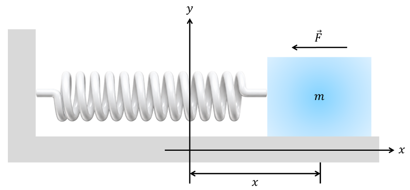
Having introduced the three formulations of mechanics, we now apply them to a simple mass–spring system to demonstrate their equivalence. As shown in Fig. 1, a block of mass

moves horizontally along the

-axis and is connected to a fixed support by a linear spring of stiffness

. The displacement

x(t)

is measured from the equilibrium position and is taken as positive to the right. Assuming a frictionless surface and neglecting the mass of the spring, the only horizontal force acting on the block is the restoring force exerted by the spring,

F=−kx(t)

. The configuration shown in Fig. 1 corresponds to a positive displacement

x(t)>0

, for which the restoring force acts in the negative

-direction. The equation of motion is derived independently using Newton’s second law, the Euler–Lagrange equation, and Hamilton’s canonical equations.

Out[]=

Fig. 1: Configuration of the mass–spring system and its coordinate system.

Derive the equation of motion using Newton’s second law:

In[]:=

newtonSpring=newtonEquations[{-kx[t]},m,{x''[t]}]

Out[]=

′′

[t]-kx[t]}

Define the kinetic energy in terms of the velocity and the potential energy in terms of the displacement:

In[]:=

SpringV=

x'[t]

Out[]=

′

[t]

In[]:=

Spring=

x[t]

Out[]=

x[t]

Construct the Lagrangian:

In[]:=

lagrangianSpring=SpringV-Spring

Out[]=

x[t]

′

[t]

Derive the equation of motion using the Euler–Lagrange equation:

In[]:=

lagrangeSpring=lagrangeEquations[lagrangianSpring,{x[t]},t]

Out[]=

′′

[t]-kx[t]}

Calculate the conjugate momentum:

In[]:=

pSpring=D[lagrangianSpring,x'[t]]

Out[]=

′

[t]

Solve for the velocity in terms of the conjugate momentum:

In[]:=

vSpring=First@Solve[p[t]==pSpring,x'[t]]

Out[]=



′

[t]

p[t]



Express the kinetic energy in terms of the conjugate momentum:

In[]:=

SpringP=SpringV/.vSpring

Out[]=

p[t]

Construct the Hamiltonian from its general definition (Eq. 4) and from the total mechanical energy for this conservative system (Eq. 5), and compare the results:

In[]:=

hamiltonianSpringGeneral=Expand[(p[t]x'[t]-lagrangianSpring)/.vSpring]

Out[]=

p[t]

x[t]

In[]:=

hamiltonianSpring=SpringP+Spring

Out[]=

p[t]

x[t]

In[]:=

hamiltonianSpringGeneral==hamiltonianSpring

Out[]=

True

Derive Hamilton’s canonical equations:

In[]:=

hamiltonSpring1stOrder=hamiltonEquations[hamiltonianSpring,{x[t]},{p[t]},t]

Out[]=



′

[t]

p[t]

′

[t]-kx[t]

Substitute the conjugate momentum into Hamilton’s equations:

In[]:=

hamiltonSpring=hamiltonSpring1stOrder/.p->(pSpring/.t->#&)

Out[]=

{True,m

′′

[t]-kx[t]}

Compare the equations of motion obtained from the three formulations:

In[]:=

newtonSpring[[1]]lagrangeSpring[[1]]hamiltonSpring[[2]]

Out[]=

′′

[t]-kx[t]

Out[]=

′′

[t]-kx[t]

Out[]=

′′

[t]-kx[t]

Simple Pendulum

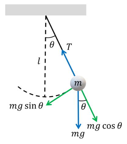
A simple pendulum provides another instructive system for comparing Newtonian, Lagrangian, and Hamiltonian mechanics. The system shown in Fig. 2 consists of a point mass

suspended from a fixed support by a massless, inextensible string of length

. Its configuration is described by the angular displacement

θ(t)

, measured from the downward vertical equilibrium position. During the motion, the mass is acted upon by the tension

along the string and its weight

. The tangential component of the weight has magnitude

mgsinθ(t)

and acts toward the equilibrium position, giving the tangential force

−mgsinθ(t)

. The fixed length of the string constrains the mass to move along a circular path, so the radial equation serves only to determine the tension and is not needed to derive the angular equation of motion. The motion is confined to a vertical plane, with friction and air resistance neglected. Small angular displacements are considered, allowing the approximation

sinθ(t)≈θ(t)

. The equation of motion is derived independently using Newton’s second law, the Euler–Lagrange equation, and Hamilton’s canonical equations.

Out[]=

Fig. 2: Configuration of the simple pendulum and the forces acting on the mass.

Derive the equation of motion using Newton’s second law and the small-angle approximation:

Define the kinetic energy in terms of the angular velocity and the potential energy in terms of the angular displacement:

Construct the Lagrangian:

Derive the equation of motion using the Euler–Lagrange equation and the small-angle approximation:

Calculate the conjugate momentum:

Solve for the velocity in terms of the conjugate momentum:

Express the kinetic energy in terms of the conjugate momentum:

Construct the Hamiltonian from its general definition (Eq. 4) and from the total mechanical energy for this conservative system (Eq. 5), and compare the results:

Derive Hamilton’s canonical equations using the small-angle approximation:

Substitute the conjugate momentum:

Compare the equations of motion obtained from the three formulations:

Atwood’s Machine

Define the dependent vertical coordinates using the constant-length constraint:

Derive Newton’s equations for the two masses:

Solve Newton’s equations for the acceleration:

Define the kinetic energy in terms of the vertical velocities and the potential energy in terms of the vertical coordinates:

Construct the Lagrangian:

Derive the equation of motion using the Euler–Lagrange equation:

Solve the Euler–Lagrange equation for the acceleration:

Calculate the conjugate momentum:

Solve for the generalized velocity in terms of the conjugate momentum:

Express the kinetic energy in terms of the conjugate momentum:

Construct the Hamiltonian from its general definition (Eq. 4) and from the total mechanical energy for this conservative system (Eq. 5), and compare the results:

Derive Hamilton’s canonical equations:

Substitute the conjugate momentum:

Solve Hamilton’s second canonical equation for the acceleration:

Compare the accelerations obtained from the three formulations:

Projectile Motion

Derive the equations of motion using Newton’s second law:

Define the kinetic energy in terms of the Cartesian velocity components and the potential energy in terms of the vertical position:

Construct the Lagrangian:

Derive the equations of motion using the Euler–Lagrange equations:

Calculate the conjugate momenta:

Solve for the velocities in terms of the conjugate momenta:

Express the kinetic energy in terms of the conjugate momenta:

Construct the Hamiltonian from its general definition (Eq. 4) and from the total mechanical energy for this conservative system (Eq. 5), and compare the results:

Derive Hamilton’s canonical equations:

Substitute the conjugate momenta:

Compare the equations of motion obtained from the three formulations:

Gravitational Central Force Field

Define the position, velocity, and acceleration vectors in Cartesian coordinates:

Define the polar unit vectors:

Define a function that resolves a Cartesian vector into its polar components:

Define the transformation from Cartesian to polar coordinates:

Express the position, velocity, and acceleration in polar components:

Derive the polar equations of motion using Newton’s second law:

Define the kinetic energy in terms of the polar velocity components and the gravitational potential energy in terms of the radial coordinate:

Construct the Lagrangian:

Derive the polar equations of motion using the Euler–Lagrange equations:

Calculate the conjugate momenta:

Solve for the generalized velocities in terms of the conjugate momenta:

Express the kinetic energy in terms of the conjugate momenta:

Construct the Hamiltonian from its general definition (Eq. 4) and from the total mechanical energy for this conservative system (Eq. 5), and compare the results:

Derive Hamilton’s canonical equations:

Substitute the conjugate momenta into Hamilton’s canonical equations:

Compare the equations of motion obtained from the three formulations:

Spherical Pendulum

Define the Cartesian coordinates of the particle in terms of the generalized coordinates θ and ϕ:

Define the speed of the particle in terms of its Cartesian velocity components:

Define the kinetic energy in terms of the generalized velocities and the gravitational potential energy in terms of the vertical position:

Construct the Lagrangian:

Derive the equations of motion using the Euler–Lagrange equations:

Calculate the conjugate momenta:

Solve for the generalized velocities in terms of the conjugate momenta:

Express the kinetic energy in terms of the conjugate momenta:

Construct the Hamiltonian from its general definition (Eq. 4) and from the total mechanical energy for this conservative system (Eq. 5), and compare the results:

Derive Hamilton’s canonical equations:

Substitute the conjugate momenta into Hamilton’s canonical equations:

Compare the equations of motion obtained from the Lagrangian and Hamiltonian formulations:

Double Pendulum

Define the speeds of the two particles in terms of their Cartesian velocity components:

Define the kinetic energy of the system in terms of the particle speeds and the gravitational potential energy in terms of their vertical positions:

Construct the Lagrangian:

Derive the coupled equations of motion using the Euler–Lagrange equations:

Calculate the conjugate momenta associated with the generalized coordinates:

Solve for the generalized velocities in terms of the conjugate momenta:

Express the kinetic energy in terms of the conjugate momenta:

Construct the Hamiltonian from its general definition (Eq. 4) and from the total mechanical energy for this conservative system (Eq. 5), and compare the results:

Derive Hamilton’s canonical equations:

Substitute the expressions for the conjugate momenta into Hamilton’s canonical equations:

Compare the equations of motion obtained from the Lagrangian and Hamiltonian formulations: