Two tanks Connected in an Interacting Fashion
Authors: Housam Binous and Ahmed Bellagi
Two tanks Connected in an Interacting Fashion
Authors: Housam Binous and Ahmed Bellagi
Authors: Housam Binous and Ahmed Bellagi
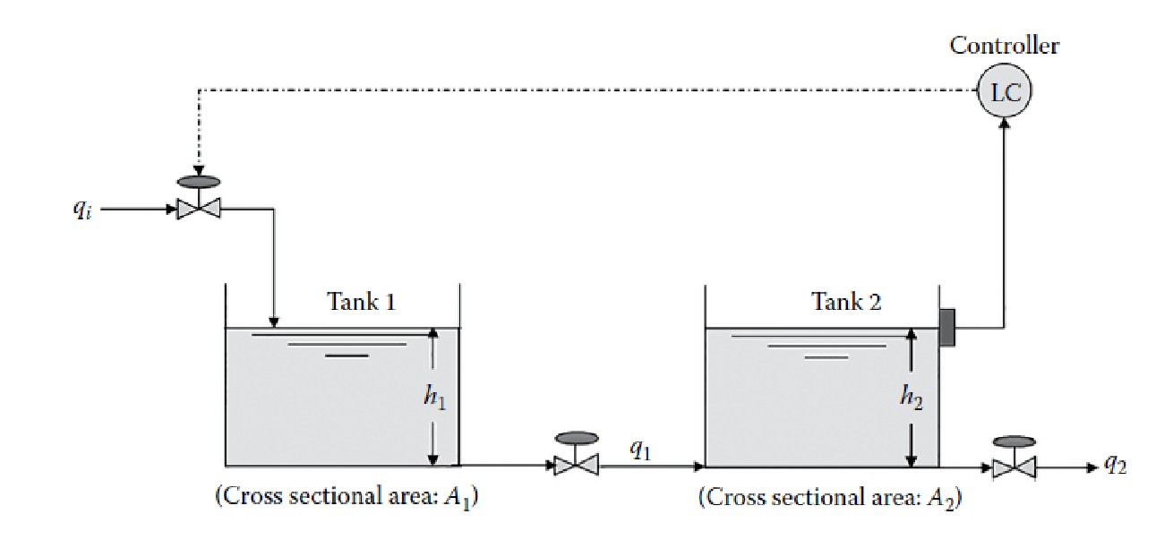
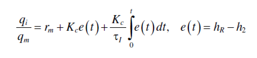
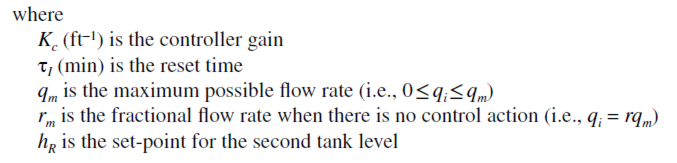
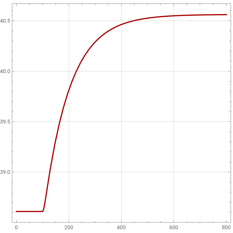
Figure below shows two tanks connected in an interacting fashion.Material balance for each tank is :When a PI controller is used, the inlet flow rate to the first tank is given byAssume the following parameters’ values : A1 = A2, C1 = 61.8 /min, C2 = 30.9 /min, hR = 6 ft, rm = 0.4, qm = 480 /min, d = 12 ft (d: tank diameter). Under such conditions, the operating point is : h1s = 48.26 ft and h2s = 38.60 ft. The fractional flow rate is increased from 0.4 to 0.41 at t=100 min to mimic a disturbance in the inlet flow rate.Plot the liquid level of each tank versus time for each one of the following scenarios :1. there is no control action.2. A P-controller is used to control the liquid level. Controller gain is Kc = 3/qm.3. A PI-controller is used to control the liquid level. Controller gain is Kc = 1/qm and the reset time is τI = 8.5 min. References:[1] Yeo, Yeong Koo, Chemical engineering computation with MATLAB, Boca Raton : Taylor & Francis, CRC Press, 2017.

2.5
ft
2.5
ft
3
ft
In[]:=
A1=A2;C1=61.8;C2=30.9;hR=6;rm=0.4;qm=480;d=12;
In[]:=
A2=Pi/4d^2//N
Out[]=
113.097
In[]:=
qi=rmqm
Out[]=
192.
In[]:=
ss=NSolve[{0qi-C1Sqrt[h1s-h2s],0C1Sqrt[h1s-h2s]-C2Sqrt[h2s]},{h1s,h2s}]
Out[]=
{{h1s48.2609,h2s38.6087}}
Open loop response or no control action
In[]:=
qi=If[t<100,rmqm,0.41qm]
Out[]=
If[t<100,rmqm,0.41qm]
In[]:=
sys={A1h1'[t]qi-C1Sqrt[h1[t]-h2[t]],A2h2'[t]C1Sqrt[h1[t]-h2[t]]-C2Sqrt[h2[t]]}
Out[]=
113.097[t]-61.8[t]61.8
′
h1
h1[t]-h2[t]
+If[t<100,rmqm,0.41qm],113.097′
h2
h1[t]-h2[t]
-30.9h2[t]
In[]:=
init={h1[0]h1s/.ss,h2[0]h2s/.ss}
Out[]=
{{h1[0]48.2609},{h2[0]38.6087}}
In[]:=
sol=NDSolve[Join[sys,init],{h1,h2},{t,0,800}]
Out[]=
h1InterpolatingFunction,h2InterpolatingFunction


In[]:=
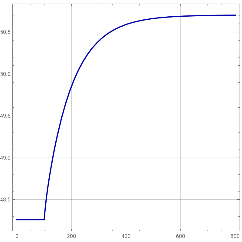
p1=Plot[h1[t]/.sol,{t,0,800},FrameTrue,GridLinesAutomatic,PlotStyle{Thick,Darker@Blue},AspectRatio1,ImageSize400{1,1}]
Out[]=
In[]:=
p2=Plot[h2[t]/.sol,{t,0,800},FrameTrue,GridLinesAutomatic,PlotStyle{Thick,Darker@Red},AspectRatio1,ImageSize400{1,1}]
Out[]=
Closed loop response - proportional only control action
In[]:=
Kc=3/qm;
In[]:=
h2sp=First[h2s/.ss]
Out[]=
38.6087
In[]:=
qi=If[t<100,rmqm,0.41qm+qmKc(h2sp-h2[t])];
Closed loop response - proportional-integral control action