ABSTRACT (original article): We study the dynamics of Friedmann-Lemaître-Robertson-Walker models where a dark energy component with a quadratic equation of state (EoS) nonlinearly interacts with cold dark matter. Thus, two energy scales naturally come into play: is the scale at which the nonlinearity of the EoS becomes relevant; is the energy scale around which the interaction starts to play an important role in the dynamics. Our focus is to understand whether there are parameter ranges for this system that can produce non-singular bouncing and emergent cosmologies for any initial condition. We complete a dynamical systems analysis, and find the parameter range such that trajectories always expand from a high energy non-singular de Sitter state. For flat and negative curvature models this de Sitter state is represented by a fixed point, the asymptotic past from which the universe emerges from. We find a subset of positive curvature models that during contraction get arbitrarily close to the de Sitter state, thus having a quasi-de Sitter bounce, then emerge from the bounce and expand, evolving toward spatial flatness. We find that the dimensionless parameter , which measures the relative strength of the nonlinear terms in the system, plays a crucial role in the topology of the phase space. When , some trajectories expand toward a singularity, while others evolve toward a low energy cosmological constant at late-times, with a subset going through a decelerated matter dominate era before the final acceleration. When , all trajectories are non-singular, and evolve toward a late-time cosmological constant. We find a subclass in this case in which all trajectories have at least one decelerated matter dominated phase, and accelerate at late-times. CITATION (original article): Molly Burkmar, Marco Bruni, Thomas Waters (2025), Singularity-free cosmology from interactions in the dark sector, arXiv:2504.01683. https://doi.org/10.48550/arXiv.2504.01683
GitHub: https://github.com/MollyBurkmar1/Interacting_Nonlinear_DE
ρ
*
ρ
i
q≡/
ρ
*
ρ
i
q<3
q>3
GitHub: https://github.com/MollyBurkmar1/Interacting_Nonlinear_DE
In this notebook, a dynamical systems analysis of an interacting dark energy scenario is completed, which is discussed in https://arxiv.org/abs/2504.01683.
Copyright © 2024 Molly Burkmar
This program is free software : you can redistribute it and/or modify it under the terms of the GNU General Public License as published by the Free Software Foundation, either version 3 of the License, or (at your option) any later version . This program is distributed in the hope that it will be useful, but WITHOUT ANY WARRANTY; without even the implied warranty of MERCHANTABILITY or FITNESS FOR A PARTICULAR PURPOSE . See the GNU General Public License for more details . You should have received a copy of the GNU General Public License along with this program . If not, see https://www.gnu.org/licenses/.
Introduction
In this notebook, we analyse a system of ODEs describing an FLRW universe with dark matter interacting with dark energy with a quadratic equation of state (EoS). The variables x, y and z in the ODEs are normalised, such that they are dimensionless, and correspond to:
x - dark energy density,
y - Hubble expansion function,
z - dark matter energy density.
We complete a dynamical systems analysis of this model to understand whether we can avoid a singularity. In addition, we want to understand whether trajectories in the phase space have a decelerated era, and a late-time accelerated expansion, as qualitatively this is consistent with observations of our Universe. Ideally, we are looking for a parameter range where all trajectories avoid a singularity and have at least one decelerated expansion phase, for any initial condition.
General Analysis
General Analysis
Manipulate Plots
Manipulate Plots
Taylor Expansion Around (1,1)
Taylor Expansion Around (1,1)
We now know the system does admit critical points representing singularities, however the behaviour of trajectories around the singularity at (1,1) is not obvious, as the numerics break down when trajectories get close enough to the singularity. We want to understand if a separatrix exists between the fixed point where X = 3/(3+q), and the critical point at (1,1). If a separatrix does exists, then some trajectories will expand to the singularity at (1,1). If it does not, then all trajectories will be non-singular.
To find if there is a separatrix to (1,1), we first Taylor expand the ODEs to second order around (1,1) and then find if an invariant line exists.
We find that when q < 3, a separatrix exists between the fixed point at X = 3/(3+q) and the critical point (1,1), however when q > 3 it does not. Therefore when q > 3, all trajectories avoid a singularity.
Define the normalised compact dynamical system for dark energy with a quadratic equation of state, X, interacting with dark matter, Z
We multiply by (1 - X) (1 - Z) so that the fixed point at (1, 1) becomes an equilibrium point and we can Taylor expand around it
We multiply by (1 - X) (1 - Z) so that the fixed point at (1, 1) becomes an equilibrium point and we can Taylor expand around it
deX=Simplify[Expand[(-3*((1-X)^2)*(X/(1-X)-ℛ)*(1+wx+ϵ*X/(1-X))-q*X*(1-X)*Z/(1-Z))*((1-X)*(1-Z))]]deZ=Simplify[Expand[(-3*Z*(1-Z)+q*X*Z*(1-Z)/(1-X))*((1-X)*(1-Z))]]
Out[]=
(-1+X)(3(1+wx)(-1+Z)ℛ+(3wx(-1+Z)(1+ℛ)-Z(q+3(1+ℛ)(-1+ϵ))+3(1+ℛ)(-1+ϵ))+X(3+6ℛ-3wx(-1+Z)(1+2ℛ)+Z(-3+q+3ℛ(-2+ϵ))-3ℛϵ))
2
X
Out[]=
(-3+(3+q)X)Z
2
(-1+Z)
Taylor expand deX around (1, 1) to second order
In[]:=
deX/.{Z->1,X->1}
Out[]=
0
In[]:=
Simplify[D[deX,X]/.{Z->1,X->1}]
Out[]=
0
In[]:=
Simplify[D[deX,Z]/.{Z->1,X->1}]
Out[]=
0
In[]:=
Simplify[D[deX,{X,2}]/.{Z->1,X->1}]
Out[]=
-2q
In[]:=
Simplify[D[D[deX,X],Z]/.{Z->1,X->1}]
Out[]=
-3ϵ
In[]:=
Simplify[D[deX,{Z,2}]/.{Z->1,X->1}]
Out[]=
0
Taylor expand deZ around (1, 1) to second order
In[]:=
deZ/.{Z->1,X->1}
Out[]=
0
In[]:=
Simplify[D[deZ,Z]/.{Z->1,X->1}]
Out[]=
0
In[]:=
Simplify[D[deZ,X]/.{Z->1,X->1}]
Out[]=
0
In[]:=
Simplify[D[deZ,{Z,2}]/.{Z->1,X->1}]
Out[]=
2q
In[]:=
Simplify[D[D[deZ,Z],X]/.{Z->1,X->1}]
Out[]=
0
In[]:=
Simplify[D[deZ,{X,2}]/.{Z->1,X->1}]
Out[]=
0
Define the Taylor expanded deX and deZ equations
deXTaylor[q_,ϵ_]:=X'=-q*(1-X)^2-3*ϵ*(1-X)*(1-Z)deZTaylor[q_,ϵ_]:=Z'=q*(1-Z)^2
Find if there is an invariant line to (1, 1)
Define F = Z - mX - c and differentiate for F’ = Z’ - mX’
When F’ = 0 an invariant line exists
When F’ = 0 an invariant line exists
FPrime=deZTaylor[q,ϵ]-m*deXTaylor[q,ϵ]
Out[]=
q-m(-q-3(1-X)(1-Z)ϵ)
2
(1-Z)
2
(1-X)
Subsitute Z (X) = mX + c
FPrimeX=FPrime/.Z->m*X+c
Out[]=
q-m(-q-3(1-X)(1-c-mX)ϵ)
2
(1-c-mX)
2
(1-X)
Find the coefficients of the constant, X and X^2 terms
ConstTerms=Coefficient[FPrimeX,X,0]XTerms=Coefficient[FPrimeX,X,1]XSqrdTerms=Coefficient[FPrimeX,X,2]
Out[]=
q-2cq+q+mq+3mϵ-3cmϵ
2
c
Out[]=
-4mq+2cmq-3mϵ+3cmϵ-3ϵ
2
m
Out[]=
mq+q+3ϵ
2
m
2
m
Find m and c when FPrimeX == 0
These are the m and c values for the invariant line
These are the m and c values for the invariant line
Solve[{ConstTerms==0,XTerms==0,XSqrdTerms==0},{m,c}]
Out[]=
{m0,c1},m-,c
q
q+3ϵ
2q+3ϵ
q+3ϵ
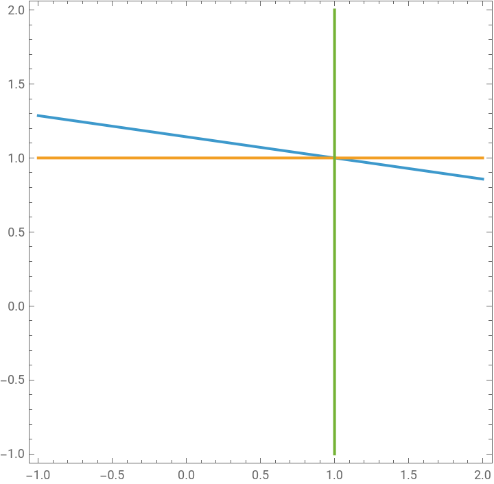
Plot the invariant line, with the boundaries X = 1 and Z = 1
For q < 3, this invariant line exists within 0 < Z, X < 1, however for q > 3, it exists outside of 0 < Z, X < 1
For q < 3, this invariant line exists within 0 < Z, X < 1, however for q > 3, it exists outside of 0 < Z, X < 1
Manipulate[ContourPlot[{Z==-q/(q+3*ϵ)*X+(2*q+3*ϵ)/(q+3*ϵ),X==1,Z==1},{Z,-1,2},{X,-1,2}],{q,0,10,Appearance->"Open"},{ϵ,-2,2,Appearance->"Open"}]
Out[]=


Flat Surface
Flat Surface
Find the Parameter Space
Find the Parameter Space
We want to find the parameter ranges for which we have a high energy repellor, as well as a low-energy attractor, such that trajectories emerge from a non-singular state, and tend towards a cosmological constant at low energy. In this section, we consider wx > -1 and wx < -1, for both ϵ = +1 and ϵ = -1. We then investigate the possible cases by varying q.
In reality, we require 10^(-120) < ℛ < 10^(-60), which corresponds to trajectories emerging between Planck and inflationary scales, however we use a much larger value to produce readable phase spaces. In the end, the dynamics is unaffected by the value of ℛ; it only affects the position of the X = ℛ/(1+ℛ) (x = ℛ) fixed point.
We find that when w > -1 and ϵ = -1, we have a phase space where the X = 3/(3+q) (x = 3/q) fixed point is a repellor, and the X = ℛ/(1+ℛ) (x = ℛ) fixed point is an attractor. The fixed point at X = (1+wx)/(1+wx-ϵ) (x = -(1+wx)/ϵ) is a saddle. Depending on the values of parameters within this range, we find that the repellor can either be a spiral repellor, a repelling node or an improper node.
In reality, we require 10^(-120) < ℛ < 10^(-60), which corresponds to trajectories emerging between Planck and inflationary scales, however we use a much larger value to produce readable phase spaces. In the end, the dynamics is unaffected by the value of ℛ; it only affects the position of the X = ℛ/(1+ℛ) (x = ℛ) fixed point.
We find that when w > -1 and ϵ = -1, we have a phase space where the X = 3/(3+q) (x = 3/q) fixed point is a repellor, and the X = ℛ/(1+ℛ) (x = ℛ) fixed point is an attractor. The fixed point at X = (1+wx)/(1+wx-ϵ)
wx < -1, ϵ = 1
wx < -1, ϵ = 1
wx < -1, ϵ = -1
wx < -1, ϵ = -1
wx > -1, ϵ = 1
wx > -1, ϵ = 1
wx > -1, ϵ = -1
wx > -1, ϵ = -1
Define ϵ
ϵ=-1;
Find wx such that the (0, ℛ) fixed point is an attractor
The eigenvalues of this point need to be negative
The eigenvalues of this point need to be negative
Reduce[-3(1+wx+ℛ*ϵ)<0&&wx>-1&&0<ℛ<1,wx]
Out[]=
0<ℛ<1&&wx>-1+ℛ
In[]:=
Reduce[-3+qℛ<0&&0<ℛ<1,q]
Find the condition such that z > 0 for the x = 3/q fixed point when (0, ℛ) is an attractor
Find the conditions on q such that the fixed point at x = 3/q is a repellor when (0, ℛ) is an attractor
Note q > 0 for this fixed point to exist at x > 0
Note q > 0 for this fixed point to exist at x > 0
Here, the assumption is that the eigenvalues are real and positive
Here the assumption is that the eigenvalues are complex with a positive real part
Here the assumption is that the eigenvalues are real, positive and the same
The x = 3/q fixed point can be a repellor for z > 0 when the x = ℛ fixed point is an attractor, but the stability of this fixed point changes depending on the combination of parameter constraints used: it can be a spiral repellor, a repelling node or an improper node. In general, there are a range of q values where both the x = ℛ and x = 3/q fixed point exist for x > 0 and z > 0, where the x = ℛ fixed point is an attractor, and the x = 3/q point is a (spiral) repellor.
Define the pressure of the dark energy
Find when the null energy condition is violated
Find when the strong energy condition is violated
Define the pressure of the dark energy in terms of compact variables
Find when Y’ > 0 when k = 0
q < 3
In this section, we analyse the dynamics when q < 3. In this case, two separatrices exist: one between the repellor and the singularity at (1,1), and the other between the repellor and saddle fixed point. These separatrices separate two types of trajectory: one group of trajectories expand towards a singularity, and the other are non-singular and tend towards the attractor fixed point representing a cosmological constant. The separatrix between the repellor and saddle fixed point is also a non-singular trajectory.
2D Phase Spaces
2D Phase Spaces
Here, we plot the 2D z - x dynamics, as well as the compact Z - X phase spaces, for wx > -1 and ϵ = -1. Y > 0 in these phase spaces, therefore the trajectories are expanding. We complete a dynamical systems analysis for each case when the repellor is a spiral repellor, a repelling node and improper node.
We also plot the curve when the acceleration is zero (a’’ = 0). The ‘curves’ in the heading below correspond to the zero acceleration curve and the separatrix between the repellor and the saddle fixed point. If the separatrix and zero acceleration curve cross, then all non-singular models, including the separatrix, have a decelerated expansion phase followed by a late-time acceleration. If the curves do not cross, then some non-singular trajectories have a decelerated phase, and some always accelerate. In this case there is one non-singular trajectory that reaches a point of zero acceleration, but otherwise accelerates. Finally, if the curves touch, then the separatrix has a point of zero acceleration, but otherwise accelerates, and all other non-singular models have a decelerated expansion phase.
First run ‘Set-Up’, then proceed to any other section.
Set-Up
Set-Up
Load MaTeX to typeset axis labels using LaTeX
Define a format style for the Z - X phase spaces
Define the colours for the fixed points
Define the dynamical system for interacting dark energy with a quadratic equation of state, x, and dark matter, z
Define the system of differential equations for the dark energy, x, and dark matter, z, in terms of a time variable
Define the compact dynamical system for interacting dark energy with a quadratic equation of state, X, and dark matter, Z
Define the compact system of differential equations for the dark energy, X, and dark matter, Z, in terms of a time variable
Plot the fixed points that arise from compactification
Find the range of q such that the (0, ℛ) fixed point is an attractor
The eigenvalues of this point need to be negative
The eigenvalues of this point need to be negative
Find the condition such that z > 0 for the x = 3/q fixed point when (0, ℛ) is an attractor
Find where the a’’ = 0 curve intercepts the x - axis
Find where one intercept is above ℛ and the other is below ℛ, so there is no late - time acceleration
We find that the two intercepts of the a’’ = 0 curve on the x-axis cannot be such that the attractor is in a deceleration period for wx > -1 and ϵ < 0. Therefore, all cases we consider have a late-time acceleration.
Find where the intercepts both cross the x - axis
For any w_x and ℛ outside this range, the acceleration curve does not cross the x-axis, but there is still late-time acceleration.
Find the conditions on q such that the fixed point at x = 3/q is a repellor when (0, ℛ) is an attractor
Here, the assumption is that the eigenvalues are real and positive
Here, the assumption is that the eigenvalues are real and positive
Find the conditions on q such that the fixed point at x = 3/q is a spiral repellor when (0, ℛ) is an attractor
Here the assumption is that the eigenvalues are complex with a positive real part
Here the assumption is that the eigenvalues are complex with a positive real part
Here the assumption is that the eigenvalues are real, positive and the same
Spiral repellor
Spiral repellor
Compact Z - X Phase Spaces: ϵ = -1
Compact Z - X Phase Spaces: ϵ = -1
Separatrix and a’’ = 0 curve cross
Clear parameter values
Set parameter values
Find the fixed points of the system
Extract the values of the fixed points and put them into one variable name
Put the fixed points into a table
Find the 2 D Jacobian matrix . D[] differentiates each expression
Find the Jacobian, eigenvalues and eigenvectors for each fixed point
Put the eigenvectors of the fixed points into a separate table
Use TableForm to display the fixed points with their Jacobian matrix, eigenvalues and eigenvectors
Plot the fixed points
Plot the phase space for the dark energy and dark matter
Plot the curves where Z’ = 0
Plot the curves where X’ = 0
Define initial conditions as a small perturbation from the saddle fixed point along the eigenvector
Solve the Z - X system around the saddle fixed point to plot the separatrix between the repellor and saddle fixed point
Plot the separatrix
Define initial conditions as a small perturbation from the repellor fixed point along the eigenvector
Solve the Z - X system around the repeller fixed point to plot the separatrix between the repellor and the singularity at (1, 1)
Plot the separatrix
Plot the boundary between accelerating and decelerating regions
Show the plots of the phase space and its components together
q > 3
In this section, we analyse the dynamics when q > 3. In this case, only one separatrix between the repellor and saddle exists, and all trajectories expand towards the attractor fixed point representing a cosmological constant, except for the separatrix which expands towards the saddle. Therefore, all trajectories are non-singular.
2D Phase Spaces
2D Phase Spaces
As before, we plot the 2D z - x dynamics, as well as the compact Z - X phase spaces, for wx > -1 and ϵ = -1. Y > 0 in these phase spaces, therefore the trajectories are expanding. We complete a dynamical systems analysis for each case when the repellor is a spiral repellor, a repelling node and improper node.
We also plot the curve when the acceleration is zero (a’’ = 0). If the separatrix and zero acceleration curve cross, then all trajectories have at least one decelerated phase. This subcase is of particular interest, as all trajectories are non-singular, and have at least one decelerated expansion phase for any initial condition. Trajectories which cross the zero acceleration curve four times have two decelerated phases, and those that cross twice have one. There is a limiting case where a trajectory first touches the zero acceleration curve, and then crosses it twice.
If the separatrix and zero acceleration curve do not cross, some trajectories have one decelerated phase, and some always accelerate. There is a limiting case where a trajectory reaches a point of zero acceleration when it touches the zero acceleration curve, but otherwise accelerates.
Finally, the separatrix and zero acceleration curve can touch. In this case, the separatrix itself is a trajectory that reaches a point of zero acceleration, but otherwise accelerates. All other trajectories cross the zero acceleration curve twice, and have once decelerated period.
First run ‘Set-Up’, then proceed to any other section.
Set-Up
Set-Up
Load MaTeX to typeset axis labels using LaTeX
Clear parameter values
Define a format style for the Z - X phase spaces
Define the colours for the fixed points
Define the dynamical system for interacting dark energy with a quadratic equation of state, x, and dark matter, z
Define the system of differential equations for the dark energy, x, and dark matter, z, in terms of a time variable
Define the compact dynamical system for interacting dark energy with a quadratic equation of state, X, and dark matter, Z
Define the compact system of differential equations for the dark energy, X, and dark matter, Z, in terms of a time variable
Plot the fixed points that arise from compactification
Find the range of q such that the (0, ℛ) fixed point is an attractor
The eigenvalues of this point need to be negative
The eigenvalues of this point need to be negative
Find the condition such that z > 0 for the x = 3/q fixed point when (0, ℛ) is an attractor
Find where the a’’ = 0 curve intercepts the x - axis
Find where one intercept is above ℛ and the other is below ℛ, so there is no late-time acceleration
We find that the two intercepts of the a’’ = 0 curve on the x-axis cannot be such that the attractor is in a deceleration period for wx > -1 and ϵ < 0. Therefore, all cases we consider have a late-time acceleration.
Find where the intercepts both cross the x-axis
For any w_x and ℛ outside this range, the acceleration curve does not cross the x-axis, but there is still late-time acceleration.
Find the conditions on q such that the fixed point at x = 3/q is a repellor when (0, ℛ) is an attractor
Here, the assumption is that the eigenvalues are real and positive
Here, the assumption is that the eigenvalues are real and positive
Find the conditions on q such that the fixed point at x = 3/q is a spiral repellor when (0, ℛ) is an attractor
Here the assumption is that the eigenvalues are complex with a positive real part
Here the assumption is that the eigenvalues are complex with a positive real part
Here the assumption is that the eigenvalues are real, positive and the same
Spiral repellor
Spiral repellor
Compact Z - X Phase Spaces: ϵ = -1
Compact Z - X Phase Spaces: ϵ = -1
Separatrix and a’’ = 0 curve cross
Clear parameter values
Set parameter values
Find the fixed points of the system
Extract the values of the fixed points and put them into one variable name
Put the fixed points into a table
Find the 2 D Jacobian matrix . D[] differentiates each expression
Find the Jacobian, eigenvalues and eigenvectors for each fixed point
Put the eigenvectors of the fixed points into a separate table
Use TableForm to display the fixed points with their Jacobian matrix, eigenvalues and eigenvectors
Plot the fixed points
Plot the phase space for the dark energy and dark matter
Plot the curves where Z’ = 0
Plot the curves where X’ = 0
Define initial conditions as a small perturbation from the saddle fixed point along the eigenvector
Solve the Z - X system around the saddle fixed point to plot the separatrix between the repellor and saddle fixed point
Plot the separatrix
Plot the boundary between accelerating and decelerating regions
Plot the fixed points that arise from compactification
Show the plots of the phase space and its components together
Plot the phase space for the dark energy and dark matter at low energy
Define a format style for the Z - X phase space zoomed in to the bottom left hand corner
Plot the phase space to show the behaviour of the trajectories at low energy
Spiral Repellor 3D Phase Spaces
Spiral Repellor 3D Phase Spaces
As before, we plot the full 3D dynamics in the case where the X = 3/(3+q) fixed point is a spiral repellor.
The ‘curves’ in the following headings refer to the separatrix and the zero acceleration (a’’ = 0) curve, and correspond to the 2D phase spaces, where there are three subcases: the curves can cross each other, touch or do not cross.
In each case, we set X0 and Z0 to define a first integral surface in the 3D phase space. We also plot the projection of the X-Y-Z phase space on the X-Z plane, which shows the trajectory in the 2D phase space that corresponds to the first integral surface plotted in 3D. We find the location and stability of the Einstein fixed points along Y = 0, and plot closed trajectories in purple, and open trajectories in blue. The Flat Friedmann Separatrix (FFS) is plotted in green, which show the flat trajectories (k = 0), and the black curves show the Closed Friedmann Separatrix (CFS), which separates different types of closed models in the phase space. The orange fixed points in the 3D phase space are at the same X-Z location as the repellor in the 2D phase space, the dark blue fixed points are at the same X-Z location as the saddle, and the magenta fixed points are at the same X-Z location as the attractor. Y > 0 corresponds to expansion, and Y < 0 to contraction.
Trajectories which bounce once contract from a low energy repelling fixed point (magenta) until they reach Y = 0 and bounce, then expand to a low energy attractor (magenta) representing a cosmological constant. Cyclic models have a bounce, and then expand until they reach a turnaround at Y = 0, where they re-collapse and bounce again at Y = 0. Expanding flat and open models emerge from a non-singular fixed point (orange), and evolve to a low energy attractor (magenta).
Begin by running ‘Set-Up’, followed by the corresponding ‘Solve the system with set parameter values’ section, before running any other sections within each chapter.
Conclusions
In this notebook, we have completed a dynamical systems analysis of dark matter interacting with dark energy with a quadratic EoS. We wanted to understand if there was a range of parameters, such that all trajectories avoid a singularity, have a decelerated expansion phase, and tend towards a cosmological constant at low energy. When ϵ = -1, wx > -1, and q > 3, we find that in the Z-X phase space all trajectories emerge from a non-singular repellor during expansion, have at least one decelerated expansion phase, and tend towards a low energy cosmological constant at late-times, for any initial condition. This is the case even if we set the parameters such that the high energy repellor is between Planck and inflationary energy scales, and the low energy attractor is close to the observed value of the cosmological constant. In the corresponding 3D phase space, open and flat models, as well as a subset of closed models which bounce once, are non-singular, and have at least one decelerated phase during expansion.
Appendix: Repellor and Improper Node 3D Phase Space Examples
Here we plot examples of the 3D phase space for both q < 3 and q > 3, for the cases where the high energy repellor is a repelling node and an improper node.
CITE THIS NOTEBOOK
CITE THIS NOTEBOOK
Singularity-free cosmology from interactions in the dark sector
by Molly Burkmar, Marco Bruni & Thomas Waters
Wolfram Community, STAFF PICKS, July 22, 2025
by Molly Burkmar, Marco Bruni & Thomas Waters
Wolfram Community, STAFF PICKS, July 22, 2025