Observer theory holds that what is perceived is a quotient of what exists; this work studies a minimal computational model of that idea. Observers are vertices of a graph whose only ability is to measure graph distance, and each vertex is assigned the tuple of its distances to the observers. Each observer set perceives the quotient graph obtained by merging vertices it cannot distinguish. Across square, hexagonal, toroidal, and random models, coordinate degeneracy proved typical, with placement mattering more than observer count. Notably, distinct observer sets never perceived the same graph, disagreeing, in every case tested, on how many vertices exist.
Introduction
Introduction
Observer Model
Observer Model
Observer theory asks what it takes to be an observer, and how the characteristics of observers shape the reality they perceive. An observer with bounded means cannot register every detail of the world, conflating many underlying states into a single perceived state; what is perceived is a quotient of what exists. This work studies a minimal model of that idea. Observers are framed minimally, as vertices of a graph whose only ability is to measure graph distance; each vertex is assigned a coordinate, given by the tuple of its distances to the observers. In Euclidean space, distances to a few reference points are enough to coordinatise the world; this is roughly how GPS works, or how two ears localise a sound. This is not always the case on a graph, where they may be neither consistent (observers may not be able to tell apart distinct vertices sharing a coordinate) nor complete (not every tuple corresponds to a vertex). The value of a minimal model is that everything becomes explicit and computable—what the observers can distinguish, the world they then construct, and when two observer sets’ constructed worlds agree. The question of a shared reality is reduced to one of graph isomorphism.
The coordinate system is given by the following association:
The coordinate system is given by the following association:
coordinates=AssociationThread[VertexList[g],Transpose@GraphDistanceMatrix[g][[VertexIndex[g,#]&/@obs,All]]]
Visualising the Collapse of Initial Graphs
Visualising the Collapse of Initial Graphs
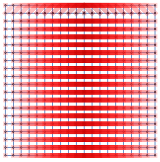
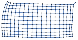
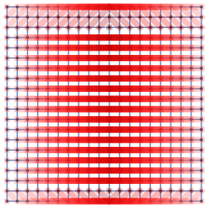
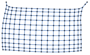
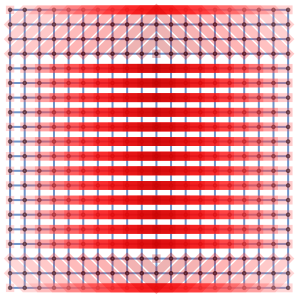
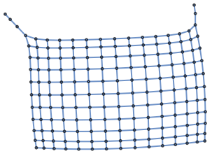
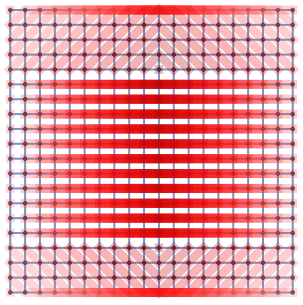
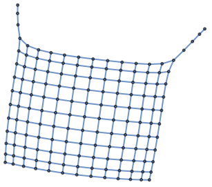
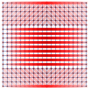
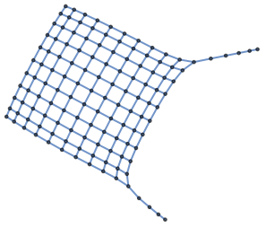
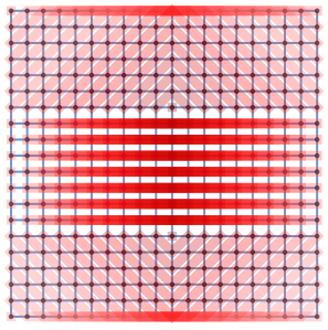
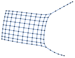
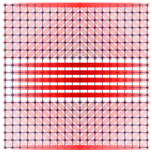
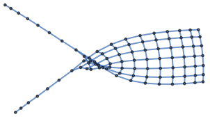
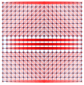
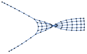
The perceived graph identifies indiscernible vertices; each edge is rewritten with its endpoints replaced by their coordinates, so vertices with the same coordinate collapse into one. A set of vertices sharing a coordinate is a fiber, highlighted in red using functions from the InfraGaugeTheory paclet. Steps of this collapse, in the case of a square lattice, are visualised below. Each row places two observers on the grid and highlights (in red) the vertices they cannot resolve. From left to right, the two observers are moved closer together, so they resolve less and the perceived graph on the right collapses to fewer and fewer vertices. The purpose of this subsection is just to show the intermediate steps in which a graph collapses; the construction is explained in greater depth before the next section, where we start with two observers before increasing the count, and later, the number of observer sets. The orientation of the perceived graphs is arbitrary: their vertices are coordinate tuples with no inherent positions, so the automatic layout chooses both placement and rotation freely. Only the shape and connectivity of the perceived graph are meaningful.
,
,
,
,
,
,
,
Further Context for Reading the Next Section
Further Context for Reading the Next Section
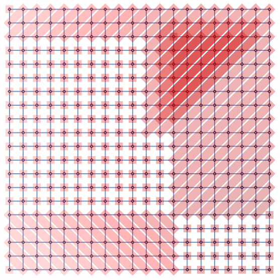
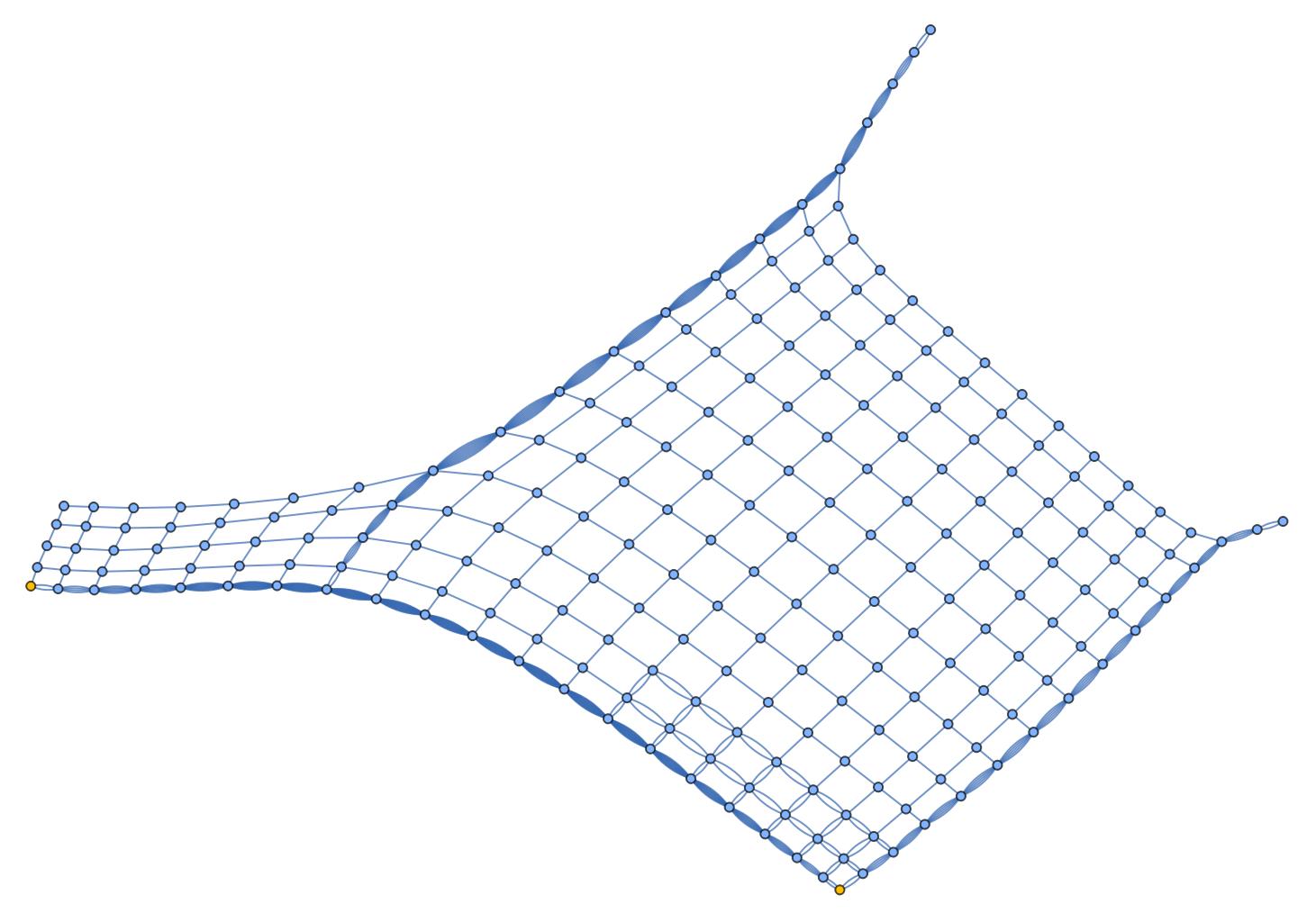
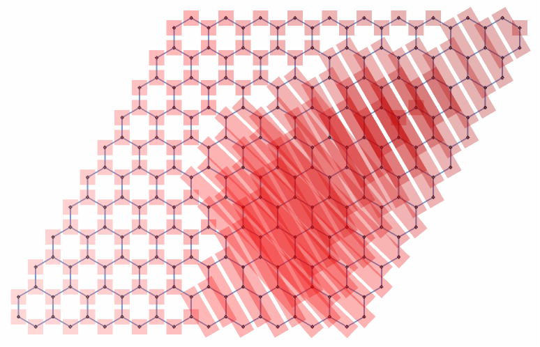
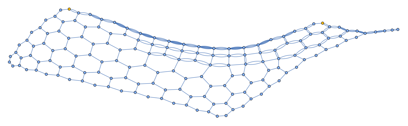
This project places observers—2 observers, 3 observers, and n-observers—on four kinds of graphs used in this project are a square lattice, hexagonal lattice, a random graph, and a toroidal grid. In every figure below, a yellow vertex marks the position of an observer. Red denotes a fiber (a set of vertices whose distances to every observer are identical). No measurement available to the observers distinguishes vertices in the same fiber. The perceived graphs (blue ones on the right) with no fibers are what remain after merging fibers into a single vertex. When a graph on the left side appears more red, it indicates that the observers were able to resolve less; more of the graph was indistinguishable to them, so more vertices were collapsed, and the perceived graph on the right is smaller and coarser. If a graph on the left had no red, it would imply that every vertex had a unique coordinate and the perceived graph matched the initial one exactly.
Observers on Graphs
Observers on Graphs
2 Observers
2 Observers
Square Lattice:
Square Lattice:
Torus:
Torus:
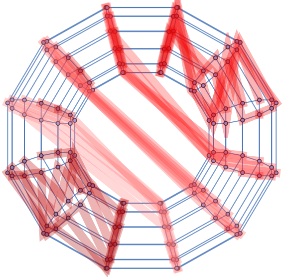
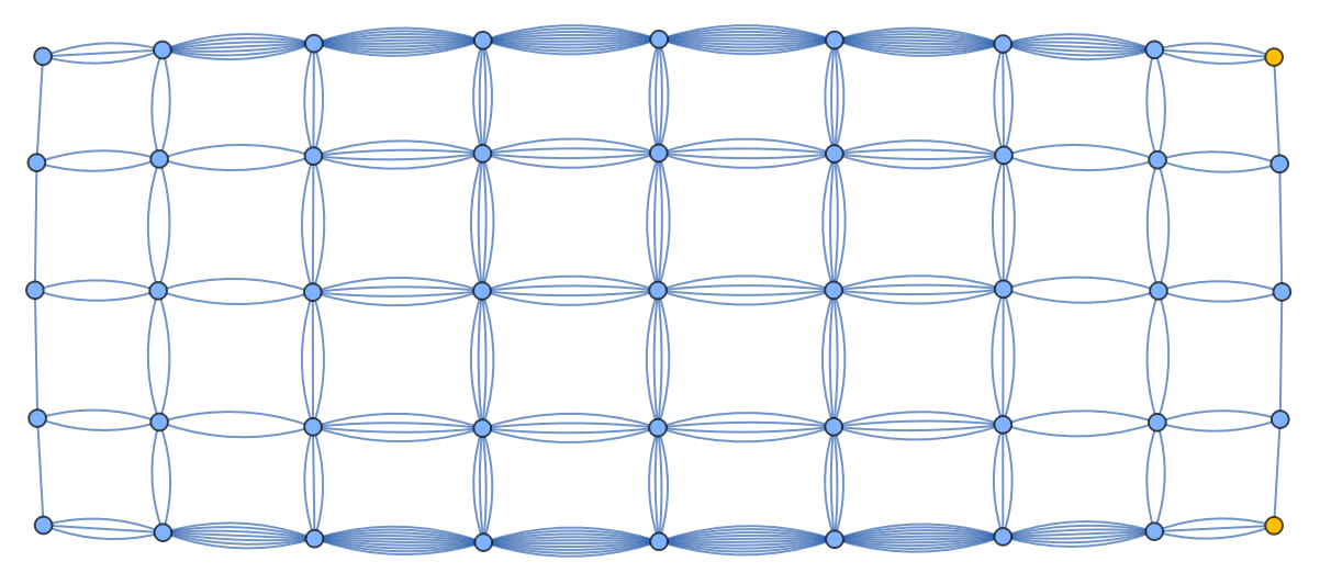
Two observers perceive the torus—a closed surface with no edge—as a flat, bounded rectangle, consistent across seeds.
Hexagonal Lattice:
Hexagonal Lattice:
Random Graph:
Random Graph:
The random graph for 2 observers is notable in that 385 vertices collapse to just 35 distinct vertices, with one fiber containing 57 of them—thus the visual noise in the centre image. With 2 random observers, structure made more of a difference than size. The square lattice and the random graph have the same vertex and edge counts but differ significantly in resolved coordinates.
Additional Observers
Additional Observers
Random Graph, 3 Observers:
Random Graph, 3 Observers:
As noted above, two observers left a 57-vertex fiber; the third observer breaks it up, but the graph still resolves only 94 of 385 coordinates with a largest fiber of 24.
Square Lattice, 3 Observers:
Square Lattice, 3 Observers:
The addition of a third observer does not shrink the largest fiber at all—the same red cluster persists from the 2 observer case. Adding an observer improved the average, but left the worst case untouched.
Hexagonal Lattice, 3 Observers:
Hexagonal Lattice, 3 Observers:
190 distinct coordinates out of 240 vertices; the largest fiber shrinks from 4 to 3. Degeneracy in the hexagonal lattice is mild relative to the other graphs.
Torus, 3 Observers:
Torus, 3 Observers:
With an additional observer, distinct coordinates increase from 45 to 106 out of 144, and the number of vertices trapped in fibers reduces from 134 to 64.
Though degenerate at 2 observers, this particular torus with 5 observers was the only graph to achieve consistency.
Square Lattice, n-Observers (2 different sets of observers):
Square Lattice, n-Observers (2 different sets of observers):
Each set of 5 observers fails to resolve a different region (in red) on the same grid; the observer sets disagree on how many vertices even exist—373 as opposed to 361.
Concluding Remarks and Future Research
Concluding Remarks and Future Research
Coordinate degeneracy was common across tests; every graph tested retained large fibers under small observer sets, and structure mattered more than size. Adding observers tended to produce diminishing returns, improving the average while sometimes leaving the largest fiber untouched. Random observers failing where two well-chosen points would succeed suggests that, as expected, localisation is a property of placement, not just observer count—i.e., two observers far apart do better to localise than three or more observers placed very close together. Distinct observer sets on the same graphs did not agree; their perceived graphs were non-isomorphic in every case tested as the different observer sets failed to agree on how many vertices exist. It might be interesting to follow up on (1) the probability of full coordinatisation as a function of observer count and graph class; (2) whether observers detect global topology, e.g., by comparing different identifications of the same local structure. Outside the context of graphs, forthcoming work with Xerxes Arsiwalla aims to provide a categorical definition of the observer, given by the unity between its minimal and maximal admissible descriptions.
Acknowledgements
Acknowledgements
I’d like to thank Xerxes Arsiwalla for overseeing this work and for a number of helpful discussions about carrying forward observer-centric work in a categorical context. I would also like to thank Pavel Hájek for his help with the code throughout the project; I could not have done this without him. The initial idea for this work belongs to Stephen Wolfram, whose early input helped to translate some research interests into the graphical project seen here.
References
References
1. D. Rickles, X. D. Arsiwalla, and H. Elshatlawy (2026), Quantum Gravity and Computation. Routledge.
2. Stephen Wolfram (2023), “Observer Theory,” writings.stephenwolfram.com/2023/12/observer-theory.
2. Stephen Wolfram (2023), “Observer Theory,” writings.stephenwolfram.com/2023/12/observer-theory.