ORIGINAL ARTICLE: Johannes Grebe-Ellis, Thomas Quick (2023), Soft shadow images, Eur. J. Phys. 44 045301.
DOI: https://doi.org/10.1088/1361-6404/acc7da
DOI: https://doi.org/10.1088/1361-6404/acc7da
Article Abstract: In traditional optics education, shadows are often regarded as a mere triviality, namely as silhouettes of obstacles to the propagation of light. However, by examining a series of shadow phenomena from an embedded perspective, we challenge this view and demonstrate how in general both the shape of the object and light source have significant impact on the resulting soft shadow images. Through experimental and mathematical analysis of the imaging properties of inverse objects, we develop a generalized concept of shadow images as complementary phenomena. Shadow images are instructive examples of optical convolution and provide an opportunity to learn about the power of embedded perspective for the study of optical phenomena in the classroom. Additionally, we introduce the less-known phenomenon of the bright shadow.
Shadow images are generally created as convolutions of the geometry of object and light source. This often leads to the surprising case that a shadow image adopt the light source geometry much more than the object. In our paper, we present a generalized description of the image conditions of the shadow. In particular, these take into account that shadows are complementary phenomena. We use Mathematica to compute the convolution products. In the figure below, on the left, we show a photographed series of shadow images generated with an L-shaped light source and inverse square shadow givers. On the right, we show the “shadow maps” calculated based on the model. The model and the assumptions made in it are explained in detail in our paper.

With the following lines we define the geometry of an L-shaped light source (Lambertian) of homogeneous radiance as a binary function, where 1 = liminous and 0 = not luminous.
In[]:=
l[x1_,x2_]:=Boole[(-1≤x1≤1&&-1≤x2≤0)||(-1≤x1≤0&&0≤x2≤1)]
Plot3D[l[x1,x2],{x1,-1.5,1.5},{x2,-1.5,1.5},PlotStyleDirective[Gray,Opacity[0.5]],PlotPoints100]

3D-Plot of the L-shaped light source
The following code shows the contour plot of the light source function. It corresponds to the view of the light source from the location of the shadow, i.e. seen from the embedded perspective.
ListContourPlot[Table[l[x1,x2],{x1,-1.5,1.5,0.01},{x2,-1.5,1.5,0.01}],ContourLinesFalse,ColorFunction"GrayTones"]
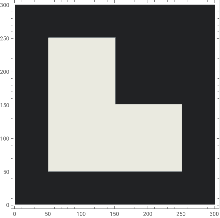
Contour plot of the L-shaped light source
Definition of the function of the object. Removing “!” in the first line generates the inverse object (obstacle <-> aperture).
In[]:=
o[x1_,x2_]:=Boole[!(-0.5≤x1≤0.5&&-0.5≤x2≤0.5)]
Plot3D[o[x1,x2],{x1,-1.5,1.5},{x2,-1.5,1.5},PlotStyleDirective[Gray,Opacity[0.5]],PlotPoints100]

3D-plot of the object
ListContourPlot[Table[o[x1,x2],{x1,-1.5,1.5,0.01},{x2,-1.5,1.5,0.01}],ContourLinesFalse,ColorFunction"GrayTones"]
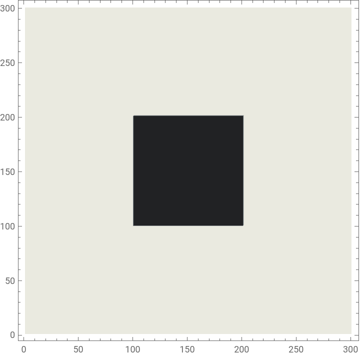
Contour plot of the object
Definition of the relative distances between object and source
In[]:=
d1=0.75;d2=0.25;
Definition of calculation steps
In[]:=
k=0.05;
Calculation of the normalized irradiance distribution of shadow images
In[]:=
lst1=ParallelTable[NIntegrate[l[x1,x2]*o[(d1*x1+d2*y1)/(d1+d2),(d1*x2+d2*y2)/(d1+d2)],{x1,-∞,∞},{x2,-∞,∞}],{y1,-5,5,k},{y2,-5,5,k}];
In[]:=
lPrependTo[lst1,ConstantArray[0,{1,Length[lst1[[1]]]}]];ListContourPlot[lst1,ContourLinesFalse,ColorFunction"GrayTones",Contours1000]
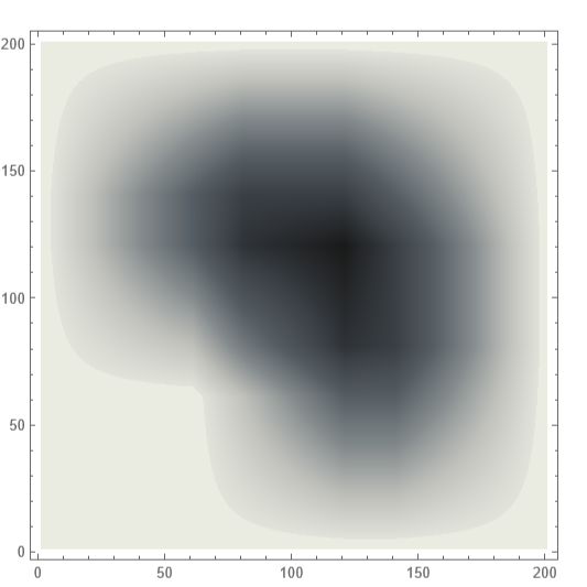
Shadow map of the quadratic object illuminated with an L-shaped light source for the given distances.
CITE THIS NOTEBOOK
CITE THIS NOTEBOOK
Soft shadow images
by Johannes Grebe-Ellis and Thomas Quick
Wolfram Community, STAFF PICKS, June 15, 2023
https://community.wolfram.com/groups/-/m/t/2938172
by Johannes Grebe-Ellis and Thomas Quick
Wolfram Community, STAFF PICKS, June 15, 2023
https://community.wolfram.com/groups/-/m/t/2938172