This study employs an SIR model to simulate a viral epidemic in a town of 300,000, considering an infection rate of and 5-day average infection duration. The model tracks susceptible, infected, recovered, and immune populations over time. Introducing treatment that shortens recovery to 1.25 days, we assess the effect of treatment initiation timing . Notably, with infections remain below 2, unlike This prompts inquiry into whether treatment alone (<1) halts transmission. Encouragingly, shows potential, suggesting the role of early treatment in controlling outbreaks.
0.6day
-1
s
(h)
h1.6,
h1.5
R
0
h1.6
Introduction
Introduction
In the town of Duckburg, a viral epidemic has been detected. The town has a population of 300,000 individuals, all of whom are currently susceptible to the virus. The outbreak began with the identification of a single infected case.
Epidemiological Parameters :
Epidemiological Parameters :
◼
Infection Rate: The infection rate is estimated to be , indicating that an infected person can transmit the virus to 60% of their susceptible contacts per day.
0.6day
-1
s
◼
Infectious Period: On average, infected individuals remain contagious for 5 days.
◼
Immunity: Upon recovery, individuals gain immunity and cannot be infected again.
Model the progression of the viral epidemic in Duckburg over a certain time period using a basic epidemiological model. Predict the number of susceptible, infected, recovered, and immune individuals at different time intervals.
Model Assumptions:
Model Assumptions:
◼
The town has a closed population with no births, deaths, or external migration during the observation period.
◼
Contacts between individuals are random, and the infection spreads uniformly in the population.
◼
The population is well-mixed, meaning that each individual has an equal chance of coming into contact with any other individual.
◼
The infectiousness of an individual is constant throughout their infectious period.
◼
Recovery results in full immunity without any loss of immunity over the observation period.
◼
Remember that this is a simplified model, and real-world epidemics can be more complex due to factors like variations in transmission rates, population demographics, and behavioral changes. The model provides a basic framework to understand the dynamics of an epidemic in a closed population.
In[]:=
Clear["Global`*"]
In[]:=
(*Parameters*)(*Recoveryrate*)γ=0.2;(*infectionrate*)β=0.6;(*FoI*)λ[t_]:=β*i[t]/n(*TotalPopulationSize*)n=300000;
(*3monthsindays*)tMax1=(0.3*365);
In[]:=
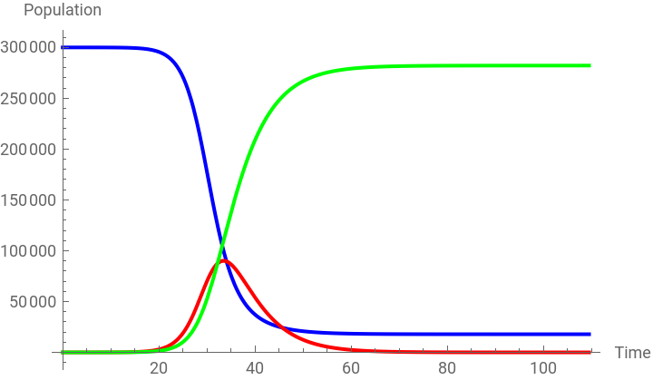
(*Definethesystemofdifferentialequations*)eqns={s'[t]==-λ[t]*s[t],i'[t]==λ[t]*s[t]-γ*i[t],r'[t]==γ*i[t],s[0]==299999,i[0]==1,r[0]==0};
In[]:=
sol=NDSolve[eqns,{s,i,r},{t,0,tMax1}];
In[]:=
Plot[Evaluate[{s[t],i[t],r[t]}/.sol],{t,0,tMax1},PlotLegends->{"Susceptible","Infected","Recovered"},AxesLabel->{"Time","Population"},AxesLabel->{"Time","Population"},PlotStyle->{Blue,Red,Green}]
Out[]=


In[]:=
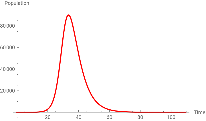
Plot[Evaluate[{i[t]}/.sol],{t,0,tMax1},PlotLegends->{"Infected"},AxesLabel->{"Time","Population"},PlotStyle->{Red},PlotRange->All]
Out[]=
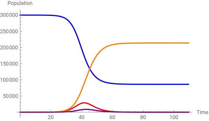
Fortunately, a treatment for the virus has been developed. While the treatment doesn’t provide instant recovery, it accelerates the healing process. On average, individuals experience recovery after 1.25 days of treatment. It’s important to note that the treatment doesn’t influence the virus’s transmission dynamics. Treated individuals remain as infectious as those who are infected but not receiving treatment.
Additionally, individuals begin receiving treatment approximately 4 days after contracting the virus. This delay between infection and treatment initiation should be considered in the model to capture the impact of the treatment on the epidemic's progression.
In[]:=
Clear["Global`*"]
In[]:=
(*Parameters*)(*Recoveryrate*)γ=0.2;(*infectionrate*)β=0.6;(*TotalPopulationSize*)n=300000;
(*therateoftreatmentinitiation*)
In[]:=
h=0.25;
(*therateofrecoveryaftertreatment*)
gammat=0.8;
(*FoI*)λ[t_]:=β*(i[t]+T[t])/n;
In[]:=
(*Definethesystemofdifferentialequations*)eqns={s'[t]==-λ[t]*s[t],i'[t]==λ[t]*s[t]-γ*i[t]-h*i[t],r'[t]==γ*i[t]+gammat*T[t],T'[t]==h*i[t]-gammat*T[t],s[0]==299999,i[0]==1,r[0]==0,T[0]==0};
In[]:=
(*3monthsindays*)tMax1=(0.3*365);
In[]:=
sol=NDSolve[eqns,{s,i,r,T},{t,0,tMax1}];
In[]:=
(*Plotthesolutions*)Plot[Evaluate[{s[t],i[t],r[t],T[t]}/.sol],{t,0,tMax1},PlotLegends->{"Susceptible","Infected","Recovered","Treated"},AxesLabel->{"Time","Population"},AxesLabel->{"Time","Population"},PlotStyle->{Blue,Red,Orange,Purple}]
Out[]=


In[]:=
Plot[Evaluate[{i[t]+T[t]}/.sol],{t,0,tMax1},PlotLegends->{"Infected +Treated"},AxesLabel->{"Time","Population"},PlotStyle->{Red},PlotRange->All]
Out[]=
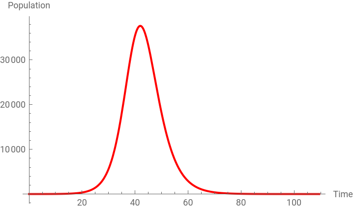
At the peak of the epidemic around 37600 are infected - this includes the 𝐼 as well as the 𝑇(treated) compartment.
In[]:=
prevalenceTable=Table[{i[t]+T[t]}/.sol,{t,0,90}];
In[]:=
(*Displaythetableofprevalencevaluesinaformattedtable*)TableForm[Transpose[{Range[0,90],prevalenceTable}],TableHeadings->{None,{"Day","Prevalence"}}]
Out[]//TableForm=
Day | Prevalence | |
0 |
| |
1 |
| |
2 |
| |
3 |
| |
4 |
| |
5 |
| |
6 |
| |
7 |
| |
8 |
| |
9 |
| |
10 |
| |
11 |
| |
12 |
| |
13 |
| |
14 |
| |
15 |
| |
16 |
| |
17 |
| |
18 |
| |
19 |
| |
20 |
| |
21 |
| |
22 |
| |
23 |
| |
24 |
| |
25 |
| |
26 |
| |
27 |
| |
28 |
| |
29 |
| |
30 |
| |
31 |
| |
32 |
| |
33 |
| |
34 |
| |
35 |
| |
36 |
| |
37 |
| |
38 |
| |
39 |
| |
40 |
| |
41 |
| |
42 |
| |
43 |
| |
44 |
| |
45 |
| |
46 |
| |
47 |
| |
48 |
| |
49 |
| |
50 |
| |
51 |
| |
52 |
| |
53 |
| |
54 |
| |
55 |
| |
56 |
| |
57 |
| |
58 |
| |
59 |
| |
60 |
| |
61 |
| |
62 |
| |
63 |
| |
64 |
| |
65 |
| |
66 |
| |
67 |
| |
68 |
| |
69 |
| |
70 |
| |
71 |
| |
72 |
| |
73 |
| |
74 |
| |
75 |
| |
76 |
| |
77 |
| |
78 |
| |
79 |
| |
80 |
| |
81 |
| |
82 |
| |
83 |
| |
84 |
| |
85 |
| |
86 |
| |
87 |
| |
88 |
| |
89 |
| |
90 |
|
Considering this, the feasibility of achieving transmission interruption solely through treatment can be assessed. Is the pace of treatment initiation achievable to achieve the goal of breaking the transmission chain?
Lets change the treatment initiation rate
Conclusion
Conclusion
CITE THIS NOTEBOOK
CITE THIS NOTEBOOK
Modeling Viral Outbreak and Treatment in a SIR Model for Duckburg
by Athanasios Paraskevopoulos
Wolfram Community, STAFF PICKS, August 31, 2023
https://community.wolfram.com/groups/-/m/t/3002391
by Athanasios Paraskevopoulos
Wolfram Community, STAFF PICKS, August 31, 2023
https://community.wolfram.com/groups/-/m/t/3002391