Explore and classify horizons in causal graphs
by Renzo Kenyi Takagui Pérez
Pontificia Universidad Católica del Perú
by Renzo Kenyi Takagui Pérez
Pontificia Universidad Católica del Perú
Abstract: Wolfram models exhibit quite explicitly event horizons through causal graphs. They are defined as a boundary to where the effects of a certain event of our interest can reach. The proposal is to use computational experiments to hunt multiway hypergraphs with the presence of horizons so that we can conjecture a way to classify them to know whether they will appear or not without a brute force approach. As a first approximation, we can use causal graphs, then if something helpful comes out of those experiments by using different rules or seeing how they evolve, we could jump into multiway hypergraphs and try the same with more intuition.
Introduction
Introduction
As in the physical world, in the Wolfram Model, we can find structures that mimic horizons. We define them as some kind of boundary where events inside can’t affect events outside. We could observe this behavior in some cases in structures called causal graphs, which are the conformal structure of spacetime for the case of hypergraphs. Trying to classify these horizons can be a bit tricky since there are many different universes in the Wolfram Model with different rules and behaviors if we evolve them. This project aims to revise some specific cases that might give us a clue on the presence of horizons as well as the use of an algorithm that will determine for us whether a causal graph contains a horizon or not.
In[]:=
ResourceFunction["WolframModel"][{{1,2},{2,3}}->{{2,3},{3,1},{4,1}},Automatic,11,"LayeredCausalGraph"]
Out[]=
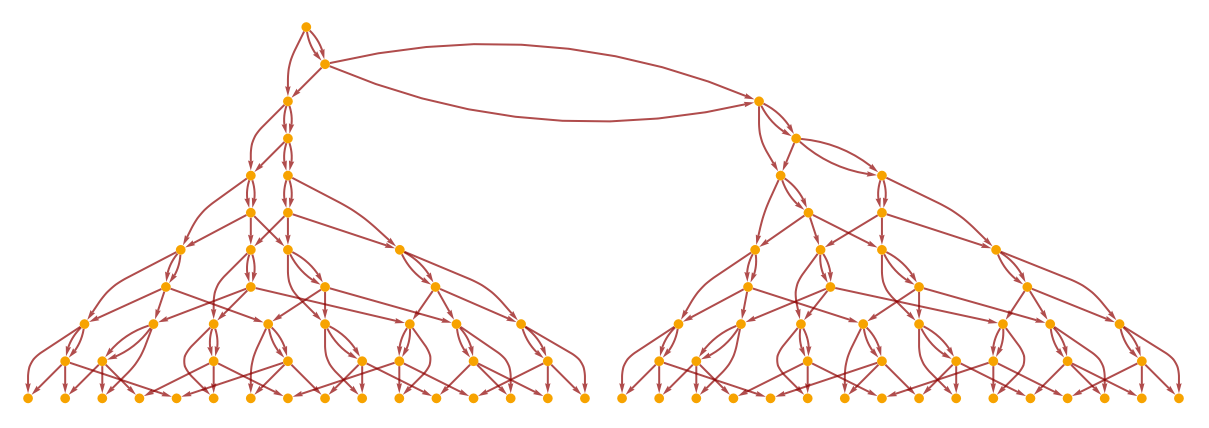
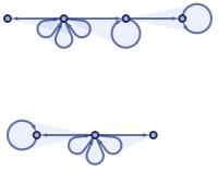
To exemplify our point, let us see a horizon in this causal graph
In[]:=
With[{gg=Graph[ResourceFunction["WolframModel"][{{1,2},{2,3}}->{{2,3},{3,1},{4,1}},Automatic,9,"LayeredCausalGraph"]]},HighlightGraph[gg,{Style[Subgraph[gg,VertexOutComponent[gg,#,10]],Red,Thick]},ImageSize->300]]&/@{3,4}
Out[]=
,
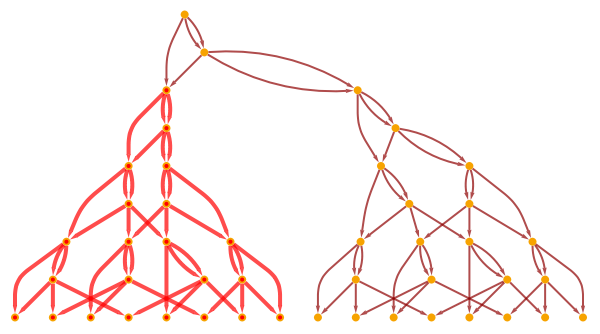
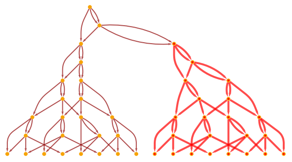
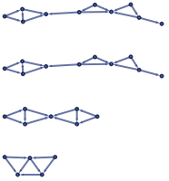
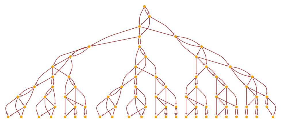
The events that happen in these two different branches cannot communicate with each other. Now, as we mentioned, the structure of the causal graph will depend on the hypergraph that is related to it. For example, if we have a disconnected hypergraph, the causal graph will show a horizon
In[]:=
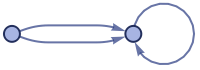
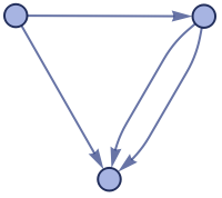
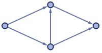
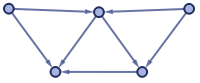
Framed[ResourceFunction["WolframModelPlot"][#,ImageSize->Tiny],FrameStyle->LightGray]&/@ResourceFunction["WolframModel"][{{1,2},{2,3}}->{{4,1},{4,2},{1,2}},Automatic,10,"StatesList"]
Out[]=
,,,,,,,,,,

In[]:=
ResourceFunction["WolframModel"][{{1,2},{2,3}}->{{4,1},{4,2},{1,2}},Automatic,12,"LayeredCausalGraph"]
Out[]=
Universe 1321
Universe 1321
In[]:=
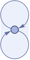
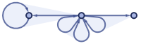
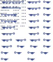
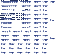
Framed[ResourceFunction["WolframModelPlot"][#,ImageSize->Tiny],FrameStyle->LightGray]&/@ResourceFunction["WolframModel"][{{{1,1,2}}->{{3,3,3},{3,3,4},{3,2,2}}},Automatic,7,"StatesList"]
Out[]=
,,,,,,,
In[]:=
ResourceFunction["WolframModel"][{{{1,1,2}}->{{3,3,3},{3,3,4},{3,2,2}}},Automatic,8,"LayeredCausalGraph"]
Out[]=

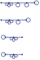
Another useful tool to analyze the emergence of horizons is the causal graph foliations, we can think of it as some kind of “time slice” in our causal graph.
In[]:=
Table[Framed[Graph[ResourceFunction["CausalConnectionGraph"][ResourceFunction["WolframModel"][{{{1,1,2}}->{{3,3,3},{3,3,4},{3,2,2}}},Automatic,#,"LayeredCausalGraph"]&,t0,12],VertexSize->.4,ImageSize->{150,30}],FrameStyle->LightGray],{t0,1,7}]
Out[]=
,,,,,,







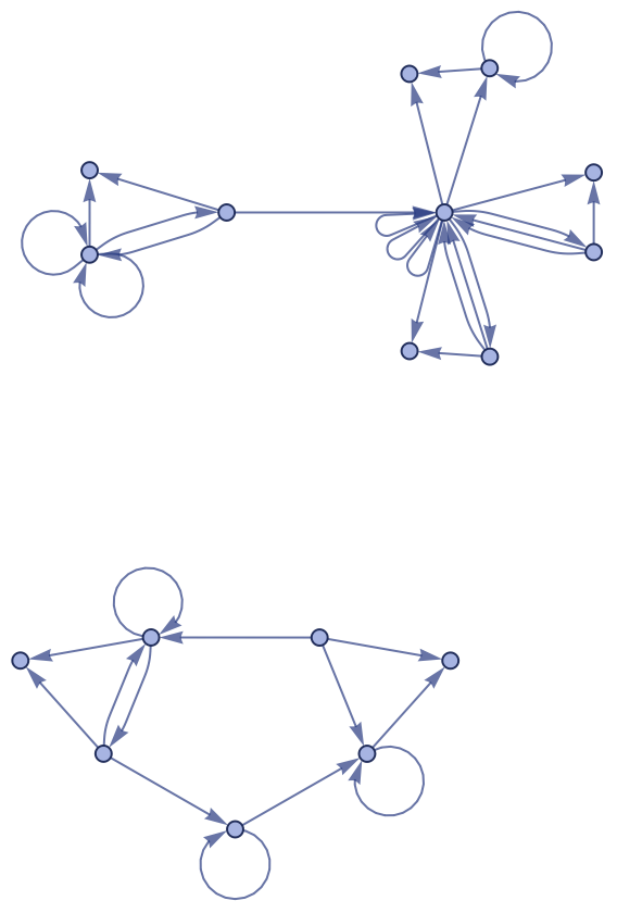
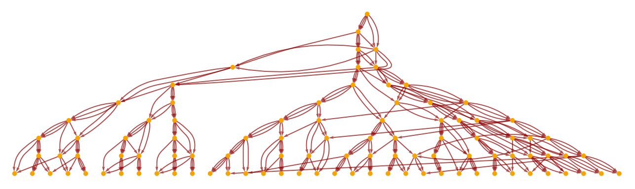
If the causal graph foliation shows more than one component in a frame, it means there is a horizon. One interesting thing to notice is that causal graphs could initially show horizons, but later on these seemingly separated branches may join again. A problem that arises to check this is that causal graphs with horizons tend to have exponential growth in the number of nodes, then tracing two branches joining again is a computationally hard task
Universe 2576
Universe 2576
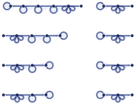
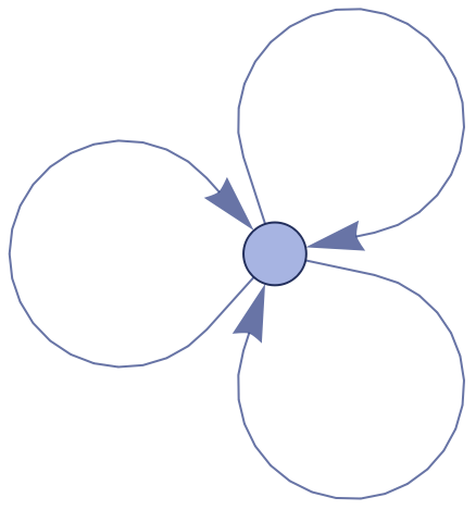
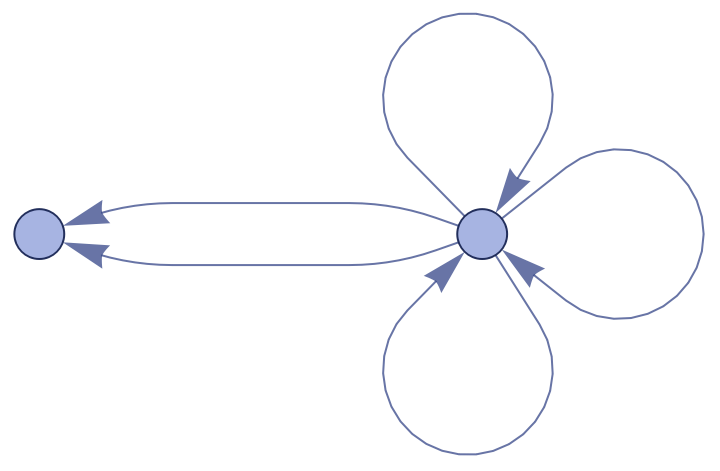
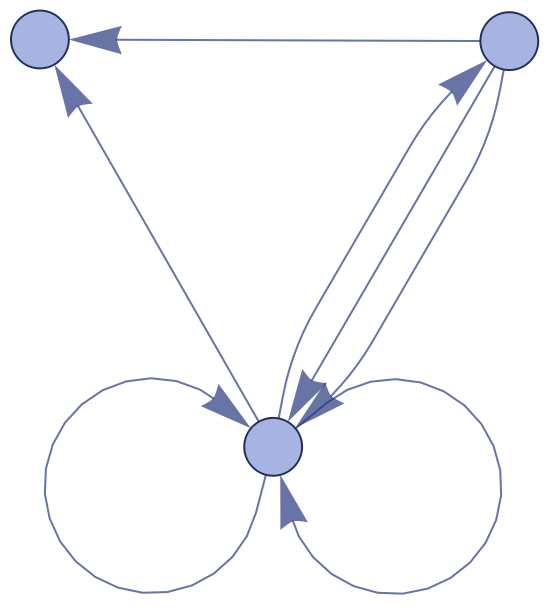
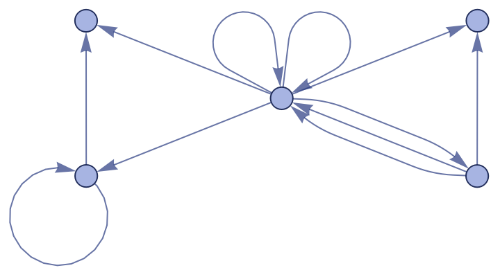
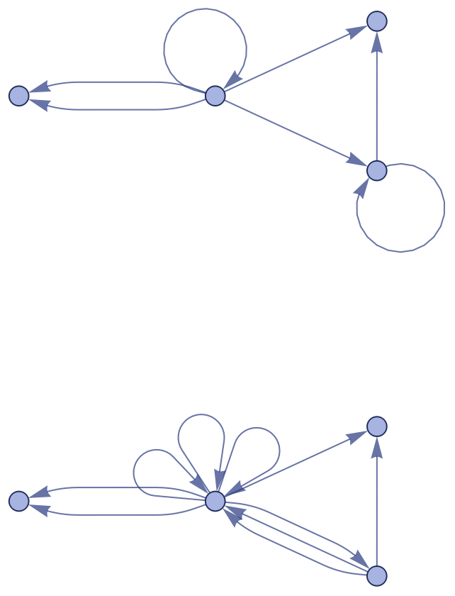
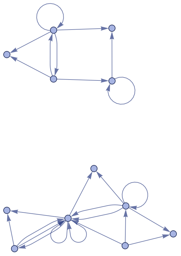
As in universe 1321, the universe 2576 maintains a one-component structure for the first steps, but later it separates, and as expected the causal graph will have a horizon. This can be easily observed in the causal graph foliations.
In[]:=
Out[]=
,
,
,
,
,
,
In[]:=
Out[]=
In[]:=
Table[Framed[Graph[ResourceFunction["CausalConnectionGraph"][ResourceFunction["WolframModel"][{{{1,2},{1,3},{1,4}}->{{2,2},{2,5},{3,2},{3,5},{3,4}}},Automatic,#,"LayeredCausalGraph"]&,t0,6],VertexSize->.4,ImageSize->{150,30}],FrameStyle->LightGray],{t0,1,6}]
Out[]=
,,,,,





Meshes and other universes
Meshes and other universes
Let us now see what happens when we consider structures that form a mesh. They usually don’t create horizons during their evolution.
Universe 1563
Universe 1563
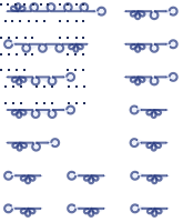
If we get the causal graph foliations, we will see there is always one component at a time.
Universe 1811
Universe 1811
This universe also exhibits only one component when we get the foliations of the causal graph. This led us to think that at least in the case of mesh-like structures there will be no horizons
Universe 1954
Universe 1954
Even though the universe 1954 doesn’t have the form of a mesh as its final state, we present it to show a usual behavior of a more random and chaotic rule.
Universe 1526
Universe 1526
Here is an example of a model that remains connected until its final state, but the causal graph has many horizons.
Different orderings
Different orderings
By having a rule, we can evolve it with many different orderings, these can have effects on the final result of its corresponding causal graph. Let us try the following rule:
{{{1,2},{1,3},{1,4}}->{{5,6},{6,7},{7,5},{5,7},{7,6},{6,5},{5,2},{6,3},{7,4},{2,7},{4,5}},{{1,2},{1,3},{1,4},{1,5}}->{{2,3},{3,4}}}
As we can observe, with different ordering we can end up with quite different hypergraphs and so with their corresponding causal graphs
For the case of “RuleIndex” and “LeastRecentEdge” there are some signs of horizons, but we expect that all of them won’t present horizons after some iterations. This is due to causal invariance.
Another example involve the rule:
{{1,2},{2,3}}->{{4,2},{4,1},{2,1},{3,4}}
If we try a different ordering the hypergraph will change as expected. Here we use “RuleOrdering”:
Again, no matter if we change the ordering because the causal graph keeps its topological form.
Articulation point algorithm
Articulation point algorithm
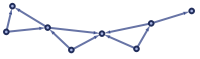
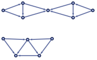
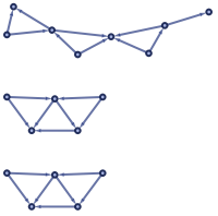
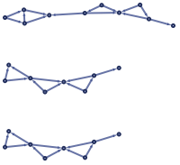
As the previous examples show, there seems to be no direct formula to determine if a certain rule will give us a horizon if we compute the causal graph. That is why we choose to apply a well-known algorithm called “articulation points” since the presence of a horizon can be detected if there is at least one node that if we remove it then the whole causal graph would separate. The idea behind the algorithm is to use a “DFS tree” which is one of the most useful techniques for solving structural problems about graphs.
DFS tree
DFS tree
We can think of the DFS tree of a graph G as its spanning tree, but the idea is how do we construct it. Run a DFS in the graph and save the edges you are passing through by omitting edges to nodes you have already visited. The edges we are saving we call them “tree-edge” or “span-edge”.
1
.Observation 1: The back-edges of the graph all connect a vertex with its descendant in the spanning tree
2
.Observation 2: A span-edge uv, where “u” and “v” are nodes, is a bridge if and only if there exists no back-edge that connects a descendant of uv with an ancestor of uv. In other words, a span-edge uv is a bridge if and only if there is no back-edge that “passes over” uv.
3
.Observation 3: A back-edge is never a bridge.
With this observations, now we can state the classical bridge-finding algorithm or articulation-point algorithm:
◼
Find the DFS tree of the graph
◼
for each span-edge uv, find out if there is a back-edge “passing over” uv, if there isn’t, you have a bridge.
This ideas can be compressed in the follow transition state:
The edge between u and its parent is a bridge if and only if dp[u]=0.
Application
Application
The application is quite straightforward since the algorithm was already implemented in the Mathematica language. Let us see what is the result for the causal graph.
There are indeed articulation points, so we say the graph has a horizon. Let us apply the algorithm for a graph we know doesn’t have a horizon.
It gives us an empty set as expected.
For the case of black hole horizons where one event can affect another, but not vice versa, the algorithm fails. The topological structure of a black hole horizon in a causal graph is somewhat different than the horizons we have been discussing.
Future directions
Future directions
The work above set up the basis for a much more general classification of horizons in causal graphs. The main focus of this project is to look for patterns and establish a function that given a causal graph as input it should tell us whether there is a horizon or not. The project was mainly focused on the classical view of the Wolfram Model, but we might expand the analysis to the quantum version.
Acknowledgments
Acknowledgments
Mentors: Xerxes Arsiwalla, Daniel Sanchez and Alessandro Pisana
References
References
◼
[1] Wolfram Physics Project: Technical Documentation. https://www.wolframphysics.org/technical-introduction/
◼
[2] Event Horizons, Singularities and Other Exotic Spacetime Phenomena, Stephen Wolfram