This notebook investigates the terminal fall velocity of a sphere across different Reynolds number regimes.
The drag coefficient is modeled using:
◼
The Schiller–Naumann correlation (1935) for Re<1000
◼
The asymptotic constant value Cd=0.44 for high Reynolds numbers
This approach allows us to explore three distinct flow regimes:
1
.Creeping flow (Re < 1) — Stokes regime
2
.Transitional regime (1 < Re < 1000)
3
.Turbulent regime (Re > 1000)
For each case, we:
◼
Solve the nonlinear differential equation governing velocity evolution using NDSolve
◼
Compute the terminal velocity using an FindRoot and steady-state formulation
◼
Compare numerical time-dependent solutions with the theoretical terminal velocity
◼
Evaluate the corresponding Reynolds number in order to check the corresponding regime assumption
The drag exhibits transitions from viscous-dominated to inertia-dominated behavior and highlights the strong coupling between velocity, Reynolds number, and drag coefficient.
This work is useful for studying particle sedimentation in fluids and can be extended to applications in suspension mechanics, fluidization, multiphase flow, and process engineering.
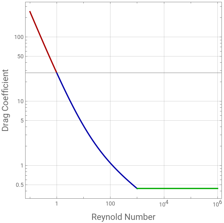
At very high Re numbers Cd=0.44 while at Re number less than 1000 one can use the Schiller-Naumann approximation:
Cd[Reynold_]:=If[Reynold==0,0,If[Reynold>1000,0.44,24/Reynold(1+0.15Reynold^0.687)]];p1=LogLogPlot[Cd[Reynold],{Reynold,10^-1,1},PlotRange->All,Frame->True,GridLines->Automatic,AspectRatio->1,PlotStyle->Darker@Red];p2=LogLogPlot[Cd[Reynold],{Reynold,1,10^3},PlotRange->All,Frame->True,GridLines->Automatic,AspectRatio->1,PlotStyle->Darker@Blue];p3=LogLogPlot[Cd[Reynold],{Reynold,10^3,10^6},PlotRange->All,Frame->True,GridLines->Automatic,AspectRatio->1,PlotStyle->Darker@Green];Show[p1,p2,p3,FrameLabel->{Style["Reynold Number",14],Style["Drag Coefficient",14]}]
Out[]=
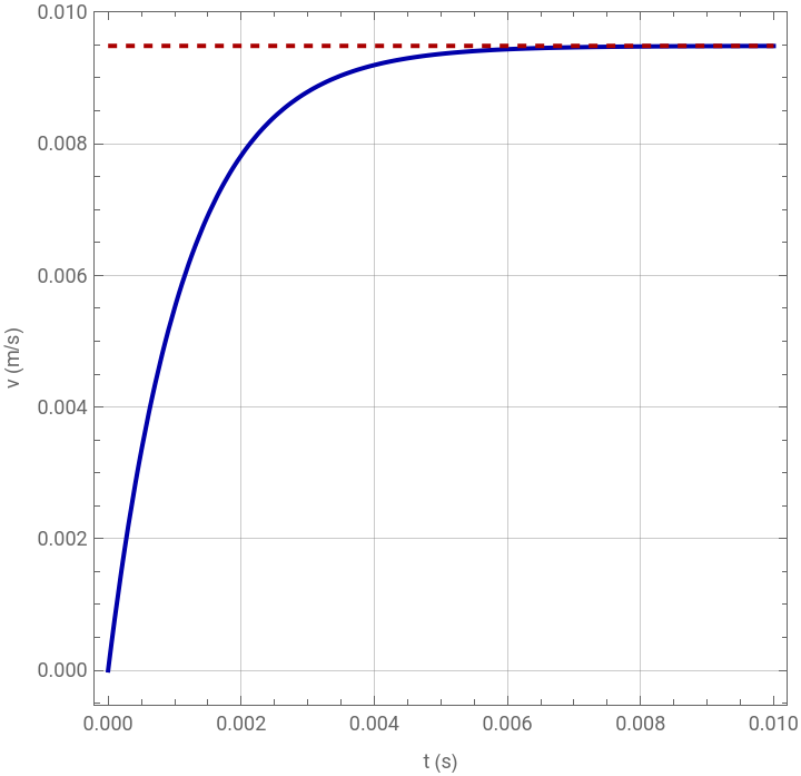
Fall velocity at Re<1 (Stokes flow)
Fall velocity at Re<1 (Stokes flow)
(*Parameters*)g=9.81;(*m/s^2*)rhoS=7800;(*spheredensitykg/m^3*)rhoF=1260;(*fluiddensitykg/m^3*)mu=1.49;(*fluidviscosityPa.s*)r=1*10^-3;(*sphereradiusm*)A=Pir^2;(*cross-sectionalarea*)
Volume:
volume=(4/3)Pir^3;
Mass:
m=rhoSvolume;
Differential equation with Re-dependent drag:
eqn=v'[t]==(mg-rhoFvolumeg-0.5rhoFACd[(2rrhoFAbs[v[t]])/mu]v[t]Abs[v[t]])/m;
Initial condition:
ic=v[0]==0;
Solve numerically:
sol=NDSolve[{eqn,ic},v,{t,0,0.01}];
Terminal velocity approximation (iterative,optional):
vTerminalApprox=v/.FindRoot[{(mg-rhoFvolumeg-0.5rhoFACd[Reynold]v^2)==0,Reynold==(2rrhoFv)/mu},{v,0.01},{Reynold,1}]
Out[]=
0.00948538
In[]:=
ReynoldApprox=Reynold/.FindRoot[{(mg-rhoFvolumeg-0.5rhoFACd[Reynold]v^2)==0,Reynold==(2rrhoFv)/mu},{v,0.01},{Reynold,1}]
Out[]=
0.0160424
Plot:
Plot[{Evaluate[v[t]/.sol],vTerminalApprox},{t,0,0.01},PlotStyle->{Darker@Blue,{Darker@Red,Dashed}},PlotLegends->{"Numerical velocity","Theoretical v_t"},FrameLabel->{"t (s)","v (m/s)"},GridLines->Automatic,PlotRange->All,AspectRatio->1,Frame->True]
Out[]=


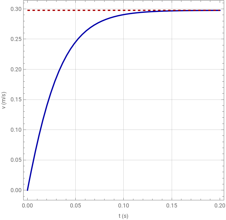
Fall velocity at 1<Re<1000 (transition regime)
Fall velocity at 1<Re<1000 (transition regime)
Parameters:
g=9.81;(*m/s^2*)rhoS=7800;(*spheredensitykg/m^3*)rhoF=1260;(*fluiddensitykg/m^3*)mu=1.4910^-2;(*fluidviscosityPa.s*)r=1*10^-3;(*sphereradiusm*)A=Pir^2;(*cross-sectionalarea*)
Volume:
volume=(4/3)Pir^3;
Mass:
m=rhoSvolume;
Terminal velocity approximation (iterative,optional):
vTerminalApprox=v/.FindRoot[{(mg-rhoFvolumeg-0.5rhoFACd[Reynold]v^2)==0,Reynold==(2rrhoFv)/mu},{v,1},{Reynold,1000}]
Out[]=
0.297652
In[]:=
ReynoldApprox=Reynold/.FindRoot[{(mg-rhoFvolumeg-0.5rhoFACd[Reynold]v^2)==0,Reynold==(2rrhoFv)/mu},{v,0.5},{Reynold,1000}]
Out[]=
50.3412
Differential equation with Re-dependent drag:
eqn=v'[t]==(mg-rhoFvolumeg-0.5rhoFACd[(2rrhoFAbs[v[t]])/mu]v[t]Abs[v[t]])/m;
Initial condition:
ic=v[0]==0;
Solve numerically:
sol=NDSolve[{eqn,ic},v,{t,0,10}];
Plot:
Plot[{Evaluate[v[t]/.sol],vTerminalApprox},{t,0,0.2},PlotStyle->{Darker@Blue,{Darker@Red,Dashed}},PlotLegends->{"Numerical velocity","Theoretical v_t"},FrameLabel->{"t (s)","v (m/s)"},GridLines->Automatic,PlotRange->All,AspectRatio->1,Frame->True]
Out[]=
Fall velocity at Re>1000 (turbulent regime)
Fall velocity at Re>1000 (turbulent regime)
Parameters:
Volume:
Mass:
Terminal velocity approximation (iterative,optional):
Differential equation with Re-dependent drag:
Initial condition:
Solve numerically:
Plot:
CITE THIS NOTEBOOK
CITE THIS NOTEBOOK
Terminal fall velocity of a sphere for various Reynolds numbers
by Housam Binous and Ahmed Bellagi
Wolfram Community, STAFF PICKS, February 9, 2026
https://community.wolfram.com/groups/-/m/t/3637039
by Housam Binous and Ahmed Bellagi
Wolfram Community, STAFF PICKS, February 9, 2026
https://community.wolfram.com/groups/-/m/t/3637039