We asked three LLM models to assist with a computational exploration, specifically OpenAI’s ChatGPT o1-pro, o1, and 4o.
TLDR: o1-pro is impressive slowly, o1 does a reasonable job quicker, 4o has become almost useless.
These were the only guiding prompts used:
Prompt 1: “can any four points in a 3D space be connected by a sphere?”
Prompt 2: “generate some code for mathematica that generates a few examples to illustrate this.”
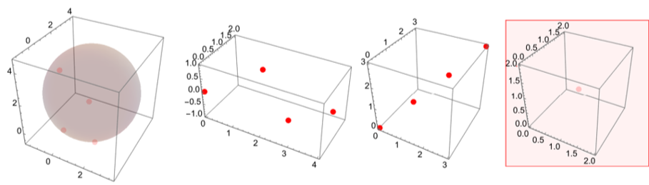
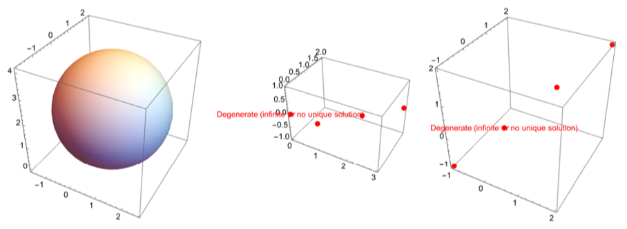
Prompt 3: “great! generate a few different examples to illustrate extreme examples. for example showing degenerate solutions making an infinite sphere etc.”
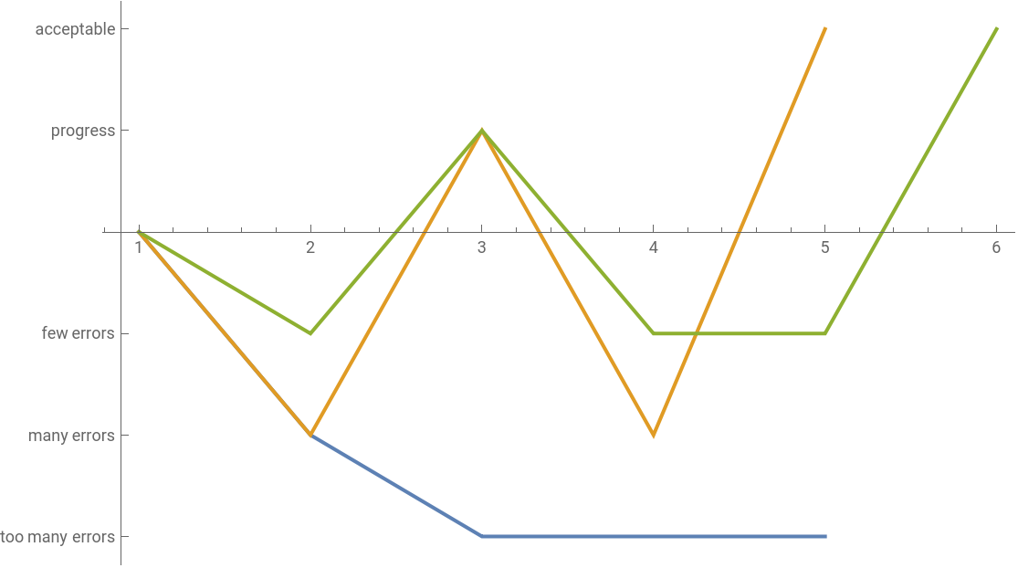
If there were any errors, we pasted those in as a direct prompt response until errors disappeared or became terrible. If the output was not satisfactory we minimally responded to get the context back on track.
Below is a plot of the responses for each model rated by satisfaction:
Out[]=


Here are the two acceptable end results for o1-pro and o1 respectively (4o was a fail):
The sections to follow are the specific responses for each agent:
o1-pro
o1-pro
In[]:=
ClearAll["Global`*"];(*Non-coplanarexample:uniquesphere*)nonCoplanarPoints={{0,0,0},{1,0,0},{0,1,0},{0,0,1}};sol1=Solve[Thread[((x-#1)^2+(y-#2)^2+(z-#3)^2)&/@nonCoplanarPoints==r^2],{x,y,z,r}];Graphics3D[{Opacity[0.2],Sphere[{x,y,z}/.sol1[[1]],r/.sol1[[1]]],Red,PointSize[Large],Point[nonCoplanarPoints]},Axes->True,PlotRange->All](*Coplanarexample:infinitesolutions*)coplanarPoints={{0,0,0},{1,0,0},{2,0,0},{3,0,0}};sol2=Solve[Thread[((x-#1)^2+(y-#2)^2+(z-#3)^2)&/@coplanarPoints==r^2],{x,y,z,r}];sol2

2
(x-#1)
2
(y-#2)
2
(z-#3)
2
(x-#1)
2
(y-#2)
2
(z-#3)
2
(x-#1)
2
(y-#2)
2
(z-#3)
2
(x-#1)
2
(y-#2)
2
(z-#3)
2
(x-#1)
2
(y-#2)
2
(z-#3)
2
(x-#1)
2
(y-#2)
2
(z-#3)
Out[]=
2
(x-#1)
2
(y-#2)
2
(z-#3)
2
(x-#1)
2
(y-#2)
2
(z-#3)
2
(x-#1)
2
(y-#2)
2
(z-#3)
2
(x-#1)
2
(y-#2)
2
(z-#3)
2
(x-#1)
2
(y-#2)
2
(z-#3)
2
(x-#1)
2
(y-#2)
2
(z-#3)
Out[]=
{}
ClearAll["Global`*"];(*Helperfunctiontogenerateequationsforpointsonasphere*)sphereEq[x_,y_,z_,pt_]:=(x-pt[[1]])^2+(y-pt[[2]])^2+(z-pt[[3]])^2(*Non-coplanarpoints:uniquesphere*)nonCoplanarPoints={{0,0,0},{1,0,0},{0,1,0},{0,0,1}};eqns1=Table[sphereEq[x,y,z,nonCoplanarPoints[[i]]]==r^2,{i,Length[nonCoplanarPoints]}];sol1=Solve[eqns1,{x,y,z,r}];Graphics3D[{Opacity[0.2],Sphere[{x,y,z}/.sol1[[1]],r/.sol1[[1]]],Red,PointSize[Large],Point[nonCoplanarPoints]},Axes->True,PlotRange->All](*Coplanarpoints:infinitelymanyspheres*)coplanarPoints={{0,0,0},{1,0,0},{2,0,0},{3,0,0}};eqns2=Table[sphereEq[x,y,z,coplanarPoints[[i]]]==r^2,{i,Length[coplanarPoints]}];sol2=Solve[eqns2,{x,y,z,r}];sol2
Out[]=

Out[]=
{}
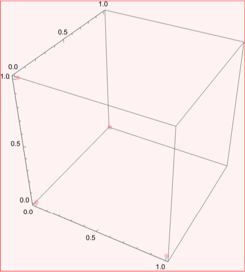
ClearAll["Global`*"];(*Helperfunctionforsphereequationsthroughpoints*)sphereEq[x_,y_,z_,pt_]:=(x-pt[[1]])^2+(y-pt[[2]])^2+(z-pt[[3]])^2(*1)Non-coplanar(uniquesphere)*)nonCoplanar={{0,0,0},{1,0,0},{0,2,0},{0,0,3}};eqns1=Table[sphereEq[x,y,z,nonCoplanar[[i]]]==r^2,{i,4}];sol1=Solve[eqns1,{x,y,z,r}];Graphics3D[{Opacity[0.2],Sphere[{x,y,z}/.sol1[[1]],r/.sol1[[1]]],Red,PointSize[Large],Point[nonCoplanar]},Axes->True](*2)Coplanar(infinitesolutions)*)coplanar={{0,0,0},{1,0,0},{2,1,0},{3,2,0}};eqns2=Table[sphereEq[x,y,z,coplanar[[i]]]==r^2,{i,4}];sol2=Solve[eqns2,{x,y,z,r}];(*3)Collinear(subsetofcoplanar,infinitesolutions)*)collinear={{0,0,0},{1,1,1},{2,2,2},{4,4,4}};eqns3=Table[sphereEq[x,y,z,collinear[[i]]]==r^2,{i,4}];sol3=Solve[eqns3,{x,y,z,r}];(*4)Allidentical(degeneratesphere,radius=0)*)identical={{1,1,1},{1,1,1},{1,1,1},{1,1,1}};eqns4=Table[sphereEq[x,y,z,identical[[i]]]==r^2,{i,4}];sol4=Solve[eqns4,{x,y,z,r}];
o1
o1
Conclusion
Conclusion
The o1 models appear to be using more advanced techniques then simple chain of thought, as demonstrated by the inferior performance of manual CoT when using 4o. o1 still holds it’s own in this context against o1-pro, and is significantly faster to respond, making o1-pro seem like overkill for this task and potentially worse. However o1-pro did avoid large numbers of errors and smartly used ClearAll first every time.
CITE THIS NOTEBOOK
CITE THIS NOTEBOOK
Chain of thought comparison for geometric reasoning in Wolfram for OpenAI's ChatGPT o1-pro, o1 & 4o
by James Wiles
Wolfram Community, STAFF PICKS, January 3, 2025
https://community.wolfram.com/groups/-/m/t/3350110
by James Wiles
Wolfram Community, STAFF PICKS, January 3, 2025
https://community.wolfram.com/groups/-/m/t/3350110