Type II Liquid Liquid Equilibrium Diagram by Common Tangent Plane and Arc-Length Continuation
Authors: Housam Binous
Type II Liquid Liquid Equilibrium Diagram by Common Tangent Plane and Arc-Length Continuation
Authors: Housam Binous
Authors: Housam Binous
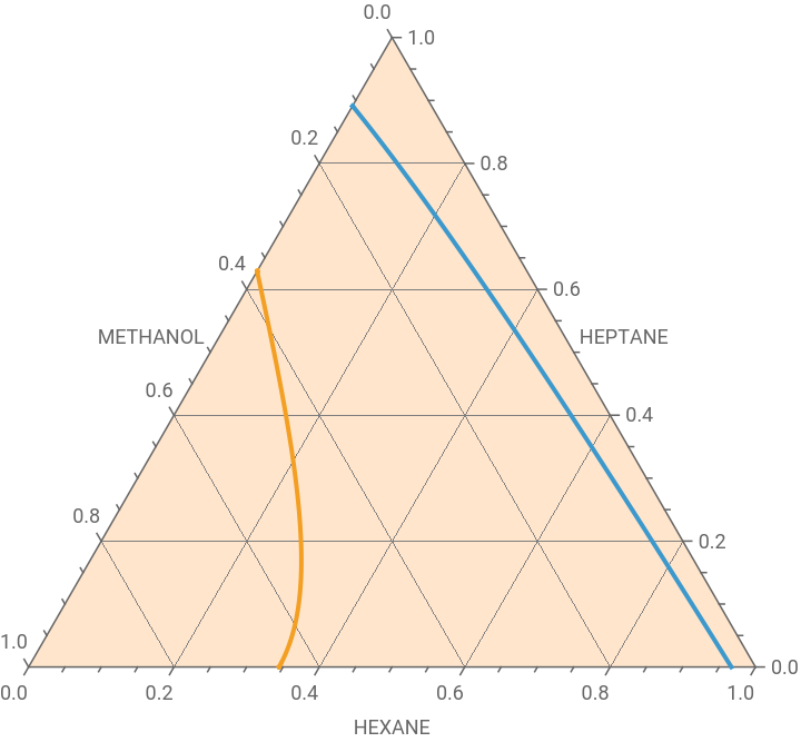
The liquid–liquid equilibrium (LLE) behavior of the methanol–hexane–heptane system at 32.85 °C was calculated using the Non-Random Two-Liquid (NRTL) activity-coefficient model combined with an arc-length continuation technique. The method was applied to the common tangent conditions derived from the Gibbs free energy of mixing, allowing the complete equilibrium boundary to be traced from a solution obtained near the critical region.
The calculation was initiated from a pair of equilibrium compositions determined by solving the common tangent equations at a specific value of the distance parameter d. These compositions served as the starting point for the continuation procedure. An arc-length constraint was introduced to transform the nonlinear equilibrium problem into a differential-algebraic system, which was then solved numerically using NDSolve. This approach enabled stable tracking of the coexistence curve over the entire heterogeneous region without loss of convergence.
The resulting ternary phase diagram exhibits Type-II liquid–liquid equilibrium behavior, characterized by an open binodal curve that intersects one side of the ternary composition triangle. Such behavior arises when one binary pair is only partially miscible, while the third component remains completely miscible with one or both of the other constituents. Consequently, the heterogeneous region extends from the binary edge into the interior of the ternary diagram rather than forming a closed loop.
The calculated binodal boundary clearly separates the single-phase and two-phase regions of the system. The smooth and continuous shape of the coexistence curve demonstrates the effectiveness of the arc-length continuation method in describing complex phase-equilibrium behavior. The results further confirm the suitability of the NRTL model for representing highly non-ideal interactions in partially miscible ternary mixtures.
Method based on common tangent plane
In[]:=
ClearAll["Global`*"];R=1.9872041;(*universalgasconstant*)T=273.15+32.85;(*temperature*)(*NRTLPARAMETERS*)a13=0.42399900;a12=0.301800;a32=0.440800;t31=1287.78000;t13=1915.07700;t23=1598.3120000;t32=1566.43700;t12=-285.9411;t21=252.997600;α={{0.,a12,a13},{a12,0.,a32},{a13,a32,0.}};τ={{0.,t12,t13},{t21,0.,t23},{t31,t32,0.}}/(RT);
In[]:=
α//MatrixForm
Out[]//MatrixForm=
0. | 0.3018 | 0.423999 |
0.3018 | 0. | 0.4408 |
0.423999 | 0.4408 | 0. |
In[]:=
τ//MatrixForm
Out[]//MatrixForm=
0. | -0.470233 | 3.14936 |
0.416057 | 0. | 2.62844 |
2.11777 | 2.57602 | 0. |
In[]:=
G[i_,j_]:=Exp[-α[[i,j]]τ[[i,j]]];(*COMPOSITIONVECTOR*)xvec[x1_,x2_]:={x1,x2,1-x1-x2};(*NRTLACTIVITYCOEFFICIENTS*)lnGamma[i_,x1_,x2_]:=Module[{x,term1,term2},x=xvec[x1,x2];term1=Sum[x[[j]]τ[[j,i]]G[j,i],{j,1,3}]/Sum[x[[k]]G[k,i],{k,1,3}];term2=Sum[x[[j]]G[i,j]/Sum[x[[k]]G[k,j],{k,1,3}](τ[[i,j]]-Sum[x[[m]]τ[[m,j]]G[m,j],{m,1,3}]/Sum[x[[m]]G[m,j],{m,1,3}]),{j,1,3}];term1+term2];gamma[i_,x1_,x2_]:=Exp[lnGamma[i,x1,x2]];(*DIMENSIONLESSGIBBSENERGYOFMIXING:g/RT*)gmix[x1_,x2_]:=Module[{x},x=xvec[x1,x2];Sum[x[[i]]Log[x[[i]]],{i,1,3}]+Sum[x[[i]]lnGamma[i,x1,x2],{i,1,3}]];(*DERIVATIVES*)dgdx1[x1_,x2_]:=Evaluate[D[gmix[u,v],u]/.{u->x1,v->x2}];dgdx2[x1_,x2_]:=Evaluate[D[gmix[u,v],v]/.{u->x1,v->x2}];(*UNKNOWNS*)vars={x1a,x2a,x1b,x2b,m1,m2};(*COMMONTANGENTEQUATIONS*)eq1=dgdx1[x1a,x2a]==m1;eq2=dgdx1[x1b,x2b]==m1;eq3=dgdx2[x1a,x2a]==m2;eq4=dgdx2[x1b,x2b]==m2;eq5=gmix[x1b,x2b]-gmix[x1a,x2a]==m1(x1b-x1a)+m2(x2b-x2a);(*EXTRACONSTRAINT-Preventtrivialsolutionxα=xβ*)eq6=(x1b-x1a)^2+(x2b-x2a)^2==d;
(*firstvalueford---verysmalld=0.07*)d0t=0.07;
In[]:=
(*solution*)(*solution*)solct=FindRoot[{eq1,eq2,eq3,eq4,eq5,eq6/.d->d0t},{{x1a,0.33},{x2a,0.4},{x1b,0.060},{x2b,0.4},{m1,-0.65},{m2,-0.45}},MaxIterations->1000]
Out[]=
{x1a0.0100149,x2a0.882978,x1b0.00706729,x2b0.618419,m1-4.54248,m20.0315688}
In[]:=
init={x1a[0]==(x1a/.solct),x2a[0]==(x2a/.solct),x1b[0]==(x1b/.solct),x2b[0]==(x2b/.solct),m1[0]==(m1/.solct),m2[0]==(m2/.solct),d[0]==d0t}
Out[]=
{x1a[0]0.0100149,x2a[0]0.882978,x1b[0]0.00706729,x2b[0]0.618419,m1[0]-4.54248,m2[0]0.0315688,d[0]0.07}
In[]:=
initdev={x1a'[0]==0.01,x2a'[0]==0.01,x1b'[0]==0.01,x2b'[0]==0.01,m1'[0]==0.01,m2'[0]==0.01,d'[0]==0.01}
Out[]=
{[0]0.01,[0]0.01,[0]0.01,[0]0.01,[0]0.01,[0]0.01,[0]0.01}
′
x1a
′
x2a
′
x1b
′
x2b
′
m1
′
m2
′
d
In[]:=
SYS={eq1,eq2,eq3,eq4,eq5,eq6}/.x1a->x1a[s]/.x1b->x1b[s]/.x2a->x2a[s]/.x2b->x2b[s]/.m1->m1[s]/.m2->m2[s]/.d->d[s];
In[]:=
Length@init
Out[]=
7
In[]:=
Length@initdev
Out[]=
7
In[]:=
Length[SYS]
Out[]=
6
In[]:=
auxeq=x1a'[s]^2+x1b'[s]^2+x2a'[s]^2+x2b'[s]^2+m1'[s]^2+m2'[s]^2+d'[s]^2==1
Out[]=
2
′
d
2
′
m1
2
′
m2
2
′
x1a
2
′
x1b
2
′
x2a
2
′
x2b
In[]:=
SYSFinal=Join[SYS,{auxeq},init,initdev];
In[]:=
Length@SYSFinal
Out[]=
21
In[]:=
SOL=NDSolve[SYSFinal,{x1a,x2a,x1b,x2b,m1,m2,d},{s,-100,100},AccuracyGoal->5]

Out[]=
x1aInterpolatingFunction,x2aInterpolatingFunction,x1bInterpolatingFunction,x2bInterpolatingFunction,m1InterpolatingFunction,m2InterpolatingFunction,dInterpolatingFunction


In[]:=
DATA1=Table[{x1a[s],x2a[s],1-x1a[s]-x2a[s]}/.SOL,{s,-7.84,16.05,0.01}];DATA2=Table[{x1b[s],x2b[s],1-x1b[s]-x2b[s]}/.SOL,{s,-7.84,16.05,0.01}];
Type II liquid-liquid equilibrium (LLE) diagram
In[]:=
p0=Show[TernaryListPlot[{Flatten[DATA1,1],Flatten[DATA2,1]},Joined->True,PlotStyle->Thick,GridLines->Automatic,FrameLabel->{"HEXANE","HEPTANE","METHANOL"},PlotRange->All,Method->{"Backdrop"->LightOrange}]]
Out[]=