Let’s define a two-level system by the time-independent Hamiltonian =+ where ϵ represents the bias (tilt) between wells, and Δ is the tunnel splitting. A classical drive in the lab frame is given by =V(t)Cos(t+ϕ) with the carrier (drive) frequency, and ϕ the carrier phase.The Rabi drive can be written as . For a π-pulse, we set it as ; thus for a sequence of square pulses with duration τ, one finds with the pulse . The overall Hamiltonian is given by
H
g
ϵ
2
σ
z
Δ
2
σ
x
H
drive
1
2
ω
d
σ
x
ω
d
Ω(t)=V(t)+
1
2
ϵ
2
Δ
2
ϵ
∫Ω(t)t=π
V(t)=Pulse
2π
τ+
ϵ
2
Δ
2
ϵ
∑
k
t-
t
k
τ
Pulse(x)=
|
|
H=+
H
g
H
drive
Define the pulse:
In[]:=
ClearAll[pulse,t];pulse[τ_,t_,tkList_]:=Sum
,{tk,tkList}
1. | 0<=t-tk<τ |
0 | True |
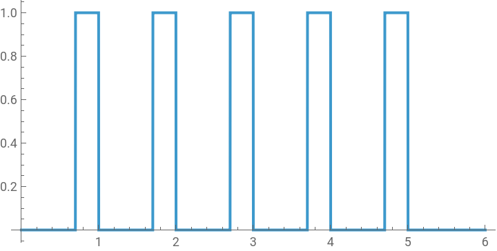
Visualize a series of pulses:
In[]:=
Plot[pulse[.3,t,Range[5]-.3],{t,0,6},Exclusions->None,AspectRatio->1/2]
Out[]=
The above behavior assumes coherent tunneling, i.e., no noise. In practice, environmental interactions introduce dephasing, relaxation, and other channels, so the dynamics deviate from the Schrödinger equation and the qubit becomes an open system. A common model for such open-system dynamics is the Lindblad master equation:
∂
t
∑
k
L
k
[][ρ]=ρ-,ρ
L
k
L
k
†
L
k
1
2
†
L
k
L
k
with the corresponding Lindblad/jump operators.
L
k
Define the Lindblad terms:
In[]:=
ClearAll[,ℒ][L_,ρ_]:=L.ρ.ConjugateTranspose[L]-(ConjugateTranspose[L].L.ρ+ρ.ConjugateTranspose[L].L)ℒ[ρ_,h_,Lk_List]:=-(h.ρ-ρ.h)+Sum[[L,ρ],{L,Lk}]
1
2
Assign values to parameters and set DEs and solve it
In[]:=
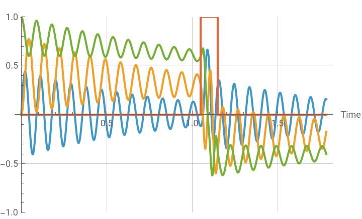
(*Timeoffirstpulse*)t0=1;(*τdurationofapulse*)τ=.1;(*Gapbetweentwopulses*)gap=1;(*timesatwhichapulseisapplied*)tk=Table[t0+τ/2+k,{k,0,gapFloor[T/gap],gap}];(*/with=+*)ratio=1;(*ϕcarrierphase*)ϕ=0;(*Δtunnelsplitting*)Δ=2π5;(*ϵbias(tilt)betweenwells*)ϵ=2π10;(*γrelaxationrate*)γ=.75;(*dephasingrate*)Γϕ=1;(*overallevolutiontime*)T=4;(*carrierdrive*)ωd=ratio+;(*Hamiltonian*)h=PauliMatrix[3]+PauliMatrix[2]+pulse[τ,t,tk]Cos[ωdt+ϕ]PauliMatrix[1];(*Lindbladoperatorswithrates*)Lk=PauliMatrix[3];(*initialdenistymatric*)ρ0=With{θ=0,ϕ=0},,Sin[θ],Sin[θ],;(*SolutionofLindbladmasterequation*)ρt=NDSolveValue[{[t]==ℒ[ρ[t],h,Lk],ρ[0]==ρ0},ρ,{t,0,T}];(*Blochvector*)vector=Re@Table[Tr[ρt[t].PauliMatrix[j]],{j,3}];ManipulateRow@Column"H=++V(t)Cos(t+ϕ)","ρ=-[H,ρ]+γ-{,ρ}+(-ρ)","withtherelaxationrateγ=1andthepuredephasingrate=1.",Plot[{vector[[1]],vector[[2]],vector[[3]],pulse[τ,t,tk]},{t,0,tf},PlotRange{-1,1},PlotLegendsPlaced[{"〈〉","〈〉","〈〉","π-pulses"},Below],ImageSizeMedium,AxesLabel{"Time",""},GridLinesAutomatic,Exclusions->None,PlotPoints->100],Show,ParametricPlot3D[vector,{t,0,tf}],ImageSize->Medium,{tf,.1T,T},SaveDefinitions:>True
ω
d
ω
p
ω
p
2
ϵ
2
Δ
Γ
ϕ
2
ϵ
2
Δ
ϵ
2
Δ
2
1
2
2π
τ+
ϵ
2
Δ
2
ϵ
γ
{{0,0},{0,1}},Γϕ
2
2
Cos
θ
2
1
2
-ϕ
1
2
ϕ
2
Sin
θ
2
′
ρ
ϵ
2
σ
z
Δ
2
σ
x
1
2
ω
d
σ
x
∂
t
σ
-
ρσ
+
1
2
σ
+
σ
-
Γ
ϕ
2
σ
z
ρσ
z
T
1
Γ
ϕ
T
ϕ
σ
x
σ
y
σ
z
Out[]=