As light passes through a fiber optic cable, most of the waves bounce off the sides, but some dissipate through the sides of the cable. However, the amount of energy dissipated greatly increases when the wave passes through a curve in the cable, as less of the light is reflected. The bend in the fiber optic cable can be modeled either as a graded index of refraction over a equivalent rectangular area, or a curved area with a graded index of refraction set by the distance from the center of the cable. When two cores are placed nearby each other in a cladding of lower index of refraction with a light input into one core, the evanescent field in that core is able to excite a wave in the other core, resulting in a swapping of the electric field between cables.
Introduction
Introduction
In today’s world, we stay connected to each other through the means of the internet. However, the amount of data that we have been sending through cables to each other has increased dramatically. In order to efficiently send this data to each other, we have been changing from coaxial data transfer cables, which propagate electric signals, to fiber optic cables, which propagate waves of light. Compared to typical coaxial cables made with metal cores, fiber optic cables are made from either glass or plastic (Optical Fiber, 2026). Light propagates through fiber optic cable by the phenomenon referred to as Total Internal Reflection (TIR) (“Total Internal Reflection”, 2026). In TIR, as light passes through an internal material and hits the external material the external material reflects it away and back into the internal substance rather than the light passing through the external material (“Total Internal Reflection”, 2026). TIR occurs when the wave speed of the light passing through the internal material is lower than the wave speed of the light passing through the external material (“Total Internal Reflection”, 2026). Since higher wave speed has a causal relation with lower index of refraction, we can classify a cable capable of TIR having a core with a higher index of refraction and a cladding with a lesser index of refraction. However, some light leaks out as it passes through the cable, with the amount depending on the angle of the refraction and specific indices of refraction of the materials composing the cable. A bend in a fiber optic cable results in a nonuniform index of refraction in the cable. In this project I will analyze the effect of a bend in a fiber optic cable on the amount energy that is lost as it passes through the cable for varying wavelengths, and use similar equations to model evanescent coupling in a fiber optic directional coupler, where the evanescent field from one cable core propagates a new wave in a nearby fiber core (“Evanescent Field”, 2026).
Using Two Different Models to Calculate Energy Loss Around the Bend
Using Two Different Models to Calculate Energy Loss Around the Bend
There are two different ways that a system can be designed to calculate the loss in energy. The first way to model energy loss is with a method that models the bent cable as a straight cable with a graded index of refraction, spanning a length of the cable equivalent to the length of the bent portion of the cable. The second way to model energy loss is by modeling the bend as it appears, a physical bend, where the index of refraction through the entire cable is dependent on the distance from the center of the core. Here it will be assumed that the power of the input is independent of the wavelength.
Loading the Finite Element Method functions for NDSolve functions:
In[]:=
<<NDSolve`FEM`
First some constants for both models can be defined, such as the light’s wavelength, it’s wavenumber, and constant index of refraction for the core and cladding materials:
In[]:=
wavelength=1.55;k0=;nCore=1.55;nClad=1.4;maxMeshSize=wavelength/(6*nCore)
2Pi
wavelength
Out[]=
0.166667
Then the size of the bent cable that we will analyze can be defined, where w0 is how narrow the energy input waveform will be. The following measurements are in µm:
In[]:=
width=10.0;w0=width/3.0;lengthStraight1=20.0;R=50.0;lengthBend=;lengthStraight2=20.0;lengthTotal=lengthStraight1+lengthBend+lengthStraight2
πR
2
Out[]=
118.54
Straight Cable with a Graded Index of Refraction Over the Curved Section
Straight Cable with a Graded Index of Refraction Over the Curved Section
Although the light is physically passing through a curved cable, we do not necessarily have to model the propagation of the light as a curve. We can instead modify the indices of refraction to be a graded index, dependent on its location relative to the center of the core. We will assume the straight core sections have a constant index of refraction.
To start we define the domain of inspection:
In[]:=
xMin=-30.0;xMax=30.0;yMin=0.0;yMax=lengthTotal;
To find index of refraction for a point, the constant index of refraction is multiplied by a gradient scalar determined by relative location (Heiblum & Harris, 1975):
Then defining the function that determines the index of reflection at a specified point:
In[]:=
nFunc[x_,y_]:=Block[{baseIndex,bendFactor},baseIndex=If[Abs[x]<=width/2,nCore,nClad];bendFactor=If[y>lengthStraight1&&y<(lengthStraight1+lengthBend),(1+x/R),1];baseIndex*bendFactor]
Visualizing the index of refraction on the domain:
In[]:=
DensityPlotnFunc[x,y],{x,xMin,xMax},{y,yMin,yMax},
Out[]=
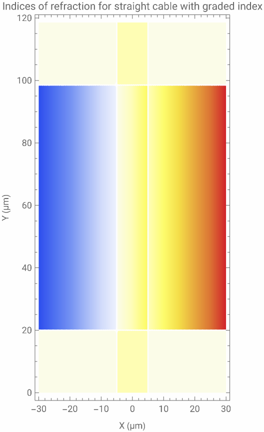
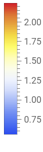
In order to calculate the wave energy at a certain position, the scalar Helmholtz partial differential equation can be used, where is the calculated wavenumber for the specified wavelength, and n is the varying index of refraction (Helmholtz Equation”, 2026). When it is solved it gives the distribution of the electric field component of the inputted polarized light:
k
0
2
∇
2
k
0
2
n
By putting a Gaussian waveform at the bottom end of the cable centered at the core, the propagation of light can be observed. While setting up the scalar Helmholtz partial differential equation, to prevent reflections off of the edges of the domain, the function NeumannValue is included.
Using the function NeumannValue to describe the behavior of the electromagnetic waves at the boundary:
In[]:=
pde=Ef[x,y]+Ef[x,y]NeumannValue[-k0nFunc[x,y]Ef[x,y],xxMin||xxMax||yyMax]+NeumannValue-k0nFunc[x,y]Ef[x,y]+2k0nFunc[x,y]Exp-,yyMin;
2
∇
{x,y}
2
k0
2
nFunc[x,y]
2
x
w0
Setting up the domain on which the partial differential equation will be solved:
In[]:=
mesh=ToElementMesh[Rectangle[{xMin,yMin},{xMax,yMax}],MaxCellMeasure->maxMeshSize];
Looking at the entire region altogether and solving the partial differential equation:
In[]:=
sol=NDSolveValue[pde,Ef,{x,y}∈mesh]
Out[]=
InterpolatingFunction


Using a density plot to visualize the electric field:
In[]:=
DensityPlotAbs[sol[x,y]],{x,xMin,xMax},{y,yMin,yMax},
Out[]=
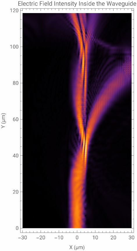
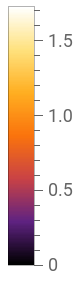
Now we have the wave, the change in energy is able to be computed.
Integrating the electric field intensity at y = 0 μm from -width/2 to width/2 for x to get the total energy of the Gaussian Mode :
In[]:=
totalEnergy=NIntegrateAbsExp-^2^2,{x,-width/2,width/2}
x
w0
Out[]=
4.16643
Then integrating the NDSolveValue at y = lengthTotal μm from -width/2 to width/2 to get the remaining energy:
In[]:=
remainingEnergy=NIntegrate[Abs[(sol[x,lengthTotal])]^2,{x,-width/2,width/2},AccuracyGoal->4]
Out[]=
1.83143
Subtracting this from the starting calculated value to get the energy lost:
In[]:=
energyLost=totalEnergy-remainingEnergy
Out[]=
2.33501
To give meaning to these arbitrary energy calculations, the energy lost can be transformed into a percentage of total energy:
In[]:=
percentLoss=100*energyLost/totalEnergy
Out[]=
56.0433
Curved Optic Fiber with Graded Index of Refraction Throughout Entire Cable
Curved Optic Fiber with Graded Index of Refraction Throughout Entire Cable
If it is desired to model the cable as it physically is, we can use Gradient-index optics, which is the study of optical effects from light passing through a material with a graded index of refraction (Gradient-Index Optics, 2025). The index of refraction for the core is a gradient dependent on the distance from the center of the cable, while the cladding has a constant index of refraction.
First the region of the curve is defined:
In[]:=
rightAngleCableCurve[cableWidth_,cableLength1_,cableLength2_]:=RegionUnion[{Rectangle[{0,(R-cableWidth)/2},{cableLength1,(R-cableWidth)/2+cableWidth}],Annulus[{cableLength1,0},{(R-cableWidth)/2,(R+cableWidth)/2},{0,Pi/2}],Rectangle[{(R-cableWidth)/2+cableLength1,-cableLength2},{(R+cableWidth)/2+cableLength1,0}]}]
Initializing the symbol cableGeometry with the region of the cable:
In[]:=
cableGeometry=rightAngleCableCurve[width,lengthStraight1,lengthStraight2]
To calculate the index of refraction with GRIN optics, a function must be defined to determine the distance of a point to the center of the core:
Visualizing the index of refraction on the domain:
Taking the helmholtz scalar partial differential equation from the previous section and make some changes to fit this model as shown below:
Looking at the entire region altogether and solving the partial differential equation:
Using a density plot to visualize the electric field:
Now we have the wave, the change in energy is able to be computed.
Integrating the electric field intensity at y = -20 μm from 50 - width/2 to 50 + width/2 for x to get the total energy of the Gaussian Mode:
Then integrating the NDSolveValue at y = lengthTotal μm from 25 - width/2 to 25 + width/2 to get the remaining energy:
Subtracting this from the starting calculated value to get the energy lost:
To give meaning to these arbitrary energy calculations, the energy lost is transformed into a percentage of total energy:
Analyzing Loss of Energy with Varying Propagated Wavelengths
Analyzing Loss of Energy with Varying Propagated Wavelengths
While a wavelength of 1.55 μm is common for the light that travels through a fiber optic cable, there are other wavelengths that are commonly used. For this reason, we should implement a function that determines the percent of energy lost depending on the wavelength of the light. We will assume that the power of the initial light inputted remains the same for all wavelengths.
Straight Cable with Graded Index of Refraction
Straight Cable with Graded Index of Refraction
In order to be able to calculate percent energy loss for a variable wavelength we must make functions that take either the wavelength or the wavenumber as a variable.
Making the wavenumber a variable in the partial differential equation for the straight cable:
Here the inputted wavelength is converted into its wavenumber for the partial differential equation:
Now we have the wave, the change in energy is able to be computed.
Then setting the integrations of the wave energies to take a wavelength variable:
Integrating the energy at the end of the cable core:
Adding the wavelength variable to the calculation of energy lost:
Adding the wavelength variable to the calculation of percent energy lost:
Generating percent energy loss from wavelengths of 0.5 μm to 1.8 μm in 0.03μm intervals:
Finally we use ListLinePlot to create a chart to show the effect of the wavelength of the light on the amount of energy that is lost as it propagates through the straightened waveguide:
Curved Optic Fiber with Graded Index of Refraction Throughout Entire Cable
Curved Optic Fiber with Graded Index of Refraction Throughout Entire Cable
Just as in the previous section, the symbols for determining change in energy will be swapped to functions that take a variable dependent on wavelength.
Making the same changes as above to the previous bent model to allow for a variable wave length:
Here converting an inputted wavelength into its wavenumber for the partial differential equation:
Now we have the wave, the change in energy is able to be computed.
Then setting the integrations of the wave energies to take a wavelength variable:
Integrating the energy at the end of the cable core:
Adding the wavelength variable to the calculation of energy lost:
Adding the wavelength variable to the calculation of percent energy lost:
Generating percent energy loss from wavelengths of 0.5 μm to 1.8 μm in 0.03 μm intervals:
Finally using ListLinePlot to create a chart to show the effect of the wavelength of the light on the amount of energy that is lost as it propagates through the curved waveguide:
Modeling a Fiber Optic Directional Coupler
Modeling a Fiber Optic Directional Coupler
So far the results have shown when two evanescent waves overlap, evanescent-wave coupling occurs. However, when evanescent-wave coupling occurs in one fiber core near another fiber core, the evanescent field can propagate a new wave in the other fiber core. This results in a passing of the wave energy between the two optical cores, in a system described as a fiber optic dynamic coupler, which will be modeled below using two models, one with a variable refractive index core and the other with a constant refractive index core.
Starting by defining/redefining some variables for a clean visualization of the phenomenon:
Next defining the regions of the dual core fiber optic cable:
We then can define the functions for applying the indices of refraction to the separate lines for both methods.
Defining the distance from core center function for the GRIN optics method:
Defining the index of refraction function for the GRIN optics method:
Defining the index of refraction for the constant core index of refraction method:
Visualizing the index of refraction on the domain for gradient index of refraction:
Visualizing the index of refraction on the domain for constant core index of refraction:
Then setting up the partial differential equation to model the energies.
For the GRIN optics method:
For the constant core index of refraction method:
Next looking at the entire region altogether, solving the partial differential equation, and plotting the results.
Solving the partial differential equation for the first model:
Solving the partial differential equation for the second model:
Plotting the energy transfer for a graded index of refraction:
Plotting the energy transfer for a constant index of refraction core:
Conclusion
Conclusion
In the first two sections, I got conflicting results on how much energy was left after the light reaches the end of the bent cable. For the straight cable model, between 40 to 100% of all of the energy was lost depending on the wave length of propagation, while for the bent cable model, between 8.4 to 100% of the energy was lost depending on the wave length propagation. However, it can be observed that on this domain the direction of the change in percent remaining energy between wavelengths is similar, such as from 1.3 to 1.8 µm, in addition to the 100% loss at 0.5 and 1.13 µm. An interesting detail of the results is that it pairs well with the wavelengths that are used in the real world. The two most common wavelengths used in fiber optic cables is 0.85, 1.3 and 1.55 µm (Fiber Optics Association, 2019). Comparing this to the energy loss per wavelength graphs, especially for the bent cable, these wavelengths align well with where the loss of energy is at it’s lowest. These models and results suggest that the most optimal way to model the transfer of energy through a bent fiber optic cable is to use gradient index optics.
In the final section, I got similar results for two different modeling systems of the fiber optic directional coupler. Both the plot for the cable with the graded refractive index core and the plot for the cable with the constant refractive index core, showed similar behavior, with both plots modeling four unique propagations in the other core. In addition, the lengths of each propagation and the distance between propagations on a single core are almost equal. Due to their similarity, I will conclude that both of these two models are valid for modeling a fiber optic directional coupler.
In the final section, I got similar results for two different modeling systems of the fiber optic directional coupler. Both the plot for the cable with the graded refractive index core and the plot for the cable with the constant refractive index core, showed similar behavior, with both plots modeling four unique propagations in the other core. In addition, the lengths of each propagation and the distance between propagations on a single core are almost equal. Due to their similarity, I will conclude that both of these two models are valid for modeling a fiber optic directional coupler.
Future Extensions
Future Extensions
In the future, other directions I could go in could include solving for the wavelength dependence of the indices of refraction, to consider the realistic response of materials used in fabrication of fiber optics. In addition, I could also consider the spectrum of a particular laser, as the input power does not have to be the same for all wavelengths, a variable I kept constant for all wavelengths in this paper. Other extensions include creating simulations for other cable geometries by using the paraxial equation and ray tracing optics inside the fiber.
Acknowledgements
Acknowledgements
I would first like to thank my Mentor Bruno Tenorio, for his exceptional assistance and thoughtful insight during the process of conducting this project. I would also like to thank the teaching assistants Hendry Xu and Daniel Xu for their amazing support throughout the program and the program directors for making this program possible.
Finally I would like to thank the person who which this research project idea stemmed from, Stephen Wolfram.
References
References
Fiber Optics Association. (2019). Understanding Wavelengths In Fiber Optics. The Fiber Optic Association, Inc. https://www.thefoa.org/tech/wavelength.htm
Heiblum, M., & Harris, J. H. (1975). Analysis of Curved Optical Waveguides by Conformal Transformation. IEEE Journal of Quantum Electronics, 11(2), 75-83.
https://www.weizmann.ac.il/condmat/heiblum/sites/condmat.heiblum/files/publications/ieee_01068563.pdf
https://www.weizmann.ac.il/condmat/heiblum/sites/condmat.heiblum/files/publications/ieee_01068563.pdf
Evanescent field. (2026, June 24). In Wikipedia. https://en.wikipedia.org/w/index.php?title=Evanescent_field&oldid=1360976416
Gradient-index optics. (2025, Sept. 24). In Wikipedia. https://en.wikipedia.org/w/index.php?title=Gradient-index_optics&oldid=1313192374
Helmholtz equation. (2026, May 17). In Wikipedia. https://en.wikipedia.org/w/index.php?title=Helmholtz_equation&oldid=1354566224
Optical fiber. (2026, June, 16). In Wikipedia. https://en.wikipedia.org/w/index.php?title=Optical_fiber&oldid=1359582532
Total internal reflection. (2026, June 29, 2026). In Wikipedia. https://en.wikipedia.org/w/index.php?title=Total_internal_reflection&oldid=1361728279
CITE THIS NOTEBOOK
CITE THIS NOTEBOOK
Modeling energy loss in a bent fiber optic cable and energy transfer by evanescent coupling
by Conrad Hostetler
Wolfram Community, STAFF PICKS, July 9, 2026
https://community.wolfram.com/groups/-/m/t/3751751
by Conrad Hostetler
Wolfram Community, STAFF PICKS, July 9, 2026
https://community.wolfram.com/groups/-/m/t/3751751