CITE THIS NOTEBOOK: Arrhenius versus exponential model for chemical reactions by Micha Peleg, Mark Normand & Maria Corradini. Wolfram Community Dec 8 2022.
ORIGINAL ARTICLE: Peleg, M., Normand, M. D., & Corradini, M. G. (2012). The Arrhenius Equation Revisited. Critical Reviews in Food Science and Nutrition, 52(9), 830–851. http://dx.doi.org/10.1080/10408398.2012.667460.
Wolfram Demonstration: http://demonstrations.wolfram.com/ArrheniusVersusExponentialModelForChemicalReactions/
Article Abstract: The Arrhenius equation has been widely used as a model of the temperature effect on the rate of chemical reactions and biological processes in foods. Since the model requires that the rate increase monotonically with temperature, its applicability to enzymatic reactions and microbial growth, which have optimal temperature, is obviously limited. This is also true for microbial inactivation and chemical reactions that only start at an elevated temperature, and for complex processes and reactions that do not follow fixed order kinetics, that is, where the isothermal rate constant, however defined, is a function of both temperature and time.
The linearity of the Arrhenius plot, that is, vs. where is in has been traditionally considered evidence of the model’s validity. Consequently, the slope of the plot has been used to calculate the reaction or processes’ “energy of activation,” usually without independent verification. Many experimental and simulated rate constant vs. temperature relationships that yield linear Arrhenius plots can also be described by the simpler exponential model . The use of the exponential model or similar empirical alternative would eliminate the confusing temperature axis inversion, the unnecessary compression of the temperature scale, and the need for kinetic assumptions that are hard to affirm in food systems. It would also eliminate the reference to the Universal gas constant in systems where a “mole” cannot be clearly identified. Unless proven otherwise by independent experiments, one cannot dismiss the notion that the apparent linearity of the Arrhenius plot in many food systems is due to a mathematical property of the model’s equation rather than to the existence of a temperature independent “energy of activation.” If in the Arrhenius model’s equation is replaced by , where the numerical value of the arbitrary constant b is substantially larger than and , the plot of vs. will always appear almost perfectly linear. Both the modified Arrhenius model version having the arbitrary constant , and the exponential model can faithfully describe temperature dependencies traditionally described by the Arrhenius equation without the assumption of a temperature independent “energy of activation.” This is demonstrated mathematically and with computer simulations, and with reprocessed classical kinetic data and published food results.
The linearity of the Arrhenius plot, that is,
Ln[k(T)]
1/T
T
°K
Ln[k(T)/k()]=c(T-)
T
reference
T
reference
T+273.16°C
T+b
T
T
reference
Lnk(T)
1/(T+b)
b,Ln[k(T)/k()=a[1/(+b)-1/(T+b)]
T
reference
T
reference
This Demonstration generates versus datasets using the Arrhenius or Arrhenius-like equations that are fitted with an exponential model. It also generates such datasets using the exponential model that are fitted by the Arrhenius or Arrhenius-like equations. The Arrhenius-like equation is presented as , where and are the rates at temperature and the reference temperature, , respectively, both in °C, and and are constants having temperature dimension. Notice that setting to 273.16 °C produces the standard Arrhenius equation. The exponential model equation is ) where is a constant having temperature reciprocal units (°).
k(T)/k()
T
ref
T
log(k(T)/k())=a(1/(+b)-1/(T+b))
T
ref
T
ref
k(T)
k()
T
ref
T
T
ref
a
b
b
log(k(T)/k())=c(T-
T
ref
T
ref
c
-1
C
The user chooses the data generation model by clicking the setter bar. The data so generated will be fitted by the other model. The number of points, , the plot's temperature range, and , the reference temperature, , and the generation or fit parameters , , and , are entered with sliders.
n
T
min
T
max
T
ref
a
b
c
The display includes the generated versus data and their fit by the opposite model (top plot) and the versus or data fitted by the opposite model (bottom plot).
k(T)/k()
T
ref
T
log(k(T)/k())
T
ref
T-
T
ref
1/(T+b)
Notice that when is large, the Arrhenius plot of the data generated by the exponential model (blue dots in bottom plot) is almost perfectly linear regardless of its absolute magnitude.
b
All curves generated by the Arrhenius equation change concavity at a high enough temperature. When the generated data has downward concavity at the chosen settings, the Demonstration forgoes the fitting by the exponential model and displays a message to that effect.
In[]:=
Out[]=


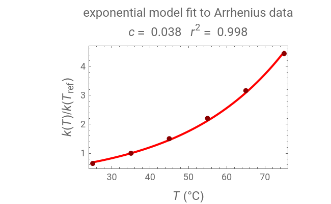
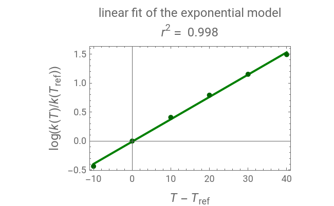
The temperature dependence of the rate of chemical reactions and biological processes is frequently described by the Arrhenius equation. This implies the existence of a log-linear relationship between the rate constant and the reciprocal of the absolute temperature, which has been used to calculate the “energy of activation”. It is shown here that there are many conditions in which data generated with a simpler exponential model can be fitted with the Arrhenius equation and vice versa. This suggests that an Arrhenius plot’s linearity is insufficient to establish that there is a temperature-independent “energy of activation” unless its existence is confirmed independently.