Cellular automata can be used as a model system for evolutionary dynamics. Here we examine how complexity is driven by selection and develop a method for extracting repeated features from patterns. By sampling square patches of patterns evolved independently under a common fitness function we look for evidence of convergent evolution.
Background
Background
A widely observed trend in the evolutionary history of life is for simple, anatomically similar organisms to develop into ones which are larger, more complex, and more diverse (Adami, 2000). For many millions of years the only life forms were very small simple bacteria (Schopf, 1993). These developed into larger and more complex single cells, before the first emergence of multicellular life around 1500MYA as coordination within colonies of unicellular individuals developed to the extent that the colony began to behave as a single organism. This process was repeated independently several times both in bacteria and eukaryotes (Bonner, 1998). Subsequently both the size and complexity of the largest multicellular life increased enormously, leading to the diversity of large complex organisms we see today.
An unresolved question is to what extent this is an active process caused by natural selection for more complex forms, or a passive one resulting in random changes resulting in an undirected drift away from an initial simple ancestor (Carroll, 2001).
Evolution can be studied experimentally using organisms which are capable of reproducing quickly such as E. Coli, used in the ongoing Long-Term Evolution Project (Lenski). Experimental methods become challenging in complex multicellular life because of the timescales involved in reproduction, making computational models a potentially useful tool to complement experimental approaches to understanding the dynamics of evolution.
Model setup
Model setup
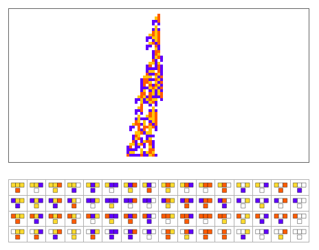
A simple model we can use to experiment with the dynamics of evolution is a 1D cellular automaton. This comprises a row of cells which can be in one of a finite number of states, together with a set of rules to update the state of each cell according to its current state and that of its neighbours.
Out[]=
Development
Development
In life the genotype encoded in DNA is translated into the phenotype by a process of development. Genes can be altered by mutation and the fitness of the phenotype to survive and reproduce determines which individuals pass their genes on to the next generation. In our model the rule set is analogous to the genotype and the development of the cell states to the phenotype.
We can model the process of evolution by choosing some function which measures the “fitness” of the CA, randomly changing one rule at each iteration, and keeping those changes which lead to a fitness as good or better than the previous ruleset (Wolfram, 2002, p. 391). This is implemented in the repository function []
We can model the process of evolution by choosing some function which measures the “fitness” of the CA, randomly changing one rule at each iteration, and keeping those changes which lead to a fitness as good or better than the previous ruleset (Wolfram, 2002, p. 391). This is implemented in the repository function []
Evolution Experiments
Evolution Experiments
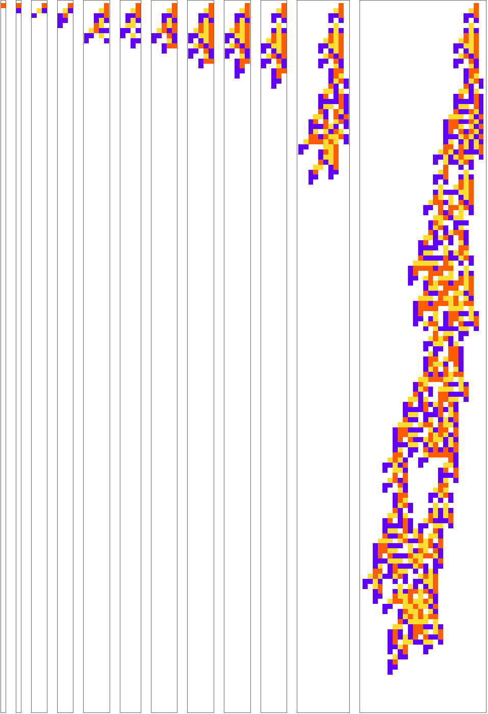
Suppose we choose lifespan as our fitness function. At each step we mutate one rule selected at random and the run the new rule set until the pattern dies out. If it runs for as long or longer than the previous record, we keep the mutation, if not, we go back to the previous rule.
Out[]=
In[]:=
data=Map[Transpose[{#[[All,"Index"]],#[[All,"BestFitness"]]}]&,lifetimeResults];ListStepPlot[data,AxesLabel->{"Step","Fitness"},PlotStyle->Directive[Blue,Opacity[0.1]],ScalingFunctions->{None,"Log"}]
Out[]=
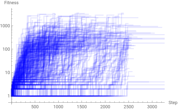
We select only rules with a fitness greater than or equal to the current best value, so fitness increases monotonically with time.
Complexity
Complexity
An important factor in understanding how evolutionary selection shapes patterns is the correlation between complexity and fitness. It is not clear to what extent increases in complexity are driven by selection pressure or by accumulated neutral mutations.
How do we measure complexity
How do we measure complexity
We have an intuitive understanding of what is meant by complexity in the context of biology, but quantifying this is a hard problem. A conceptually simple measure of the complexity of an object is the Kolmogorov complexity, defined as the shortest program which produces the object as its output. It has the advantage of being simple to define and applicable to arbitrary data, but is unable to distinguish between fine structure and random noise. The exact Kolmogorov complexity is not computable since some candidate programs will fail to terminate but we can find an upper bound using an efficient compression algorithm. Here we use the built-in function as a proxy for complexity.
Compression Methods
Compression Methods
A compression level of 1.0 will provide the best upper bound for complexity, but a simple experiment suggests reducing this to 0.95 should produce similar results in less time.
In[]:=
ListLinePlot[ParallelTable[{c,ExportByteArray[lifetimeCAs[[1,-1]],"PNG",CompressionLevel->c]//Length},{c,0,1,0.1}],AxesLabel->{"compression level","size"}]
Out[]=
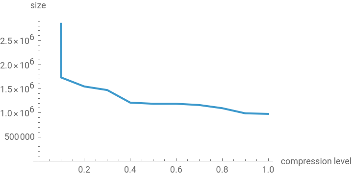
In practice the built-in Compress function provide a quick alternative.
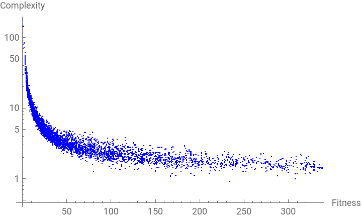
The question we would like to answer is whether patterns produced by rules evolved under a fitness function are more complex than those generated at random. A scatter plot of complexity against fitness for a set of 500 evolutionary trajectories reveals complexity decreases rapidly as repeated structures emerge.
Complexity
Complexity
The complexity of the pattern relative to its area decreases as it grows due to the emergence of repeated structures.
Out[]=
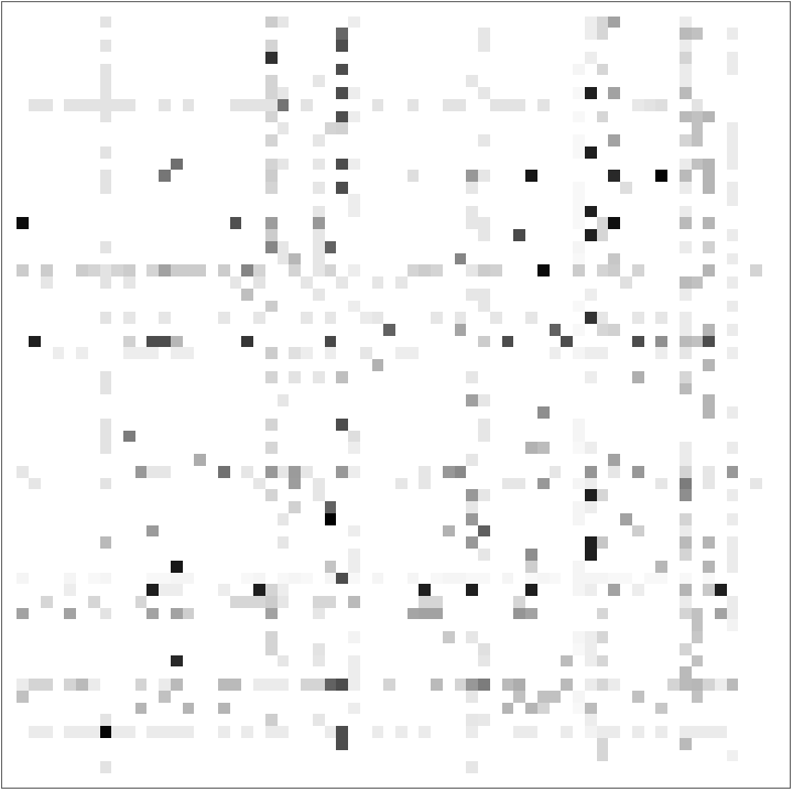
We can measure to what extent complexity depends on fitness by comparing this with rules mutated at random. The plot below shows the effects on fitness of simultaneously mutating pairs of rule cases from a CA selected for lifespan. We can select those which don’t die out immediately to measure the effects of random mutation.
Out[]=
Out[]=
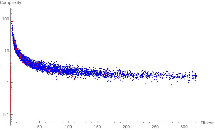
Here trajectories under selection are plotted in blue, and random mutations are plotted in red.
It would appear that complexity is reduced as a function of fitness for random mutations, but we need more data to be able to tell if this effect is genuine.
It would appear that complexity is reduced as a function of fitness for random mutations, but we need more data to be able to tell if this effect is genuine.
Patterns
Patterns
The overall pattern of this CA is complex but we can readily identify some structures and repeated patterns such as the yellow and blue terminal components. To study the evolution of diversity it is useful to automate the process of identifying repeated structures. A simple way to do this is to extract square patches which share common elements. Not all features are square so we match on any shape which touches the borders of the tile. Non matching pixels are indicated in black.
Most common tiles
Most common tiles
Let us examine the most common patches from the same CA illustrated above.
The histogram shows the counts of the most 10 most abundant 4x4 patches. Here the dominant features are the terminal structures running down the left hand side. This is counterintuitive since one might expect that in a CA optimised for maximum lifetime, the terminal elements would be where evolved mechanisms break down, and so would have less in common than elements of the rest of the pattern. One possible explanation is that branches which don’t terminate will interfere with the main body of the pattern.
Convergent evolution
Convergent evolution
The plot shows the correlation between a reference trajectory evolved under selection for lifespan and a sample of independent trajectories evolved under the same fitness function. With an initial zero rule for each trajectory, correlation scores begin at the maximum possible and then fall dramatically as the different rulesets accumulate random mutations. Correlation then gradually increases as the CA approaches optimal fitness, suggesting convergence on some common mechanisms.
If we compare this plot (blue) with the correlation between the same reference trajectory and a sample of trajectories selected for width(red), we see a similar trend but with a lower average correlation.
CAs evolved under the same fitness function show a greater structural correlation than those with different fitness functions. This suggests there may be some degree of convergent evolution, where the same mechanism which is particularly well suited to some purpose emerges independently in different species.
Discussion and Conclusions
Discussion and Conclusions
Adaptive cellular automaton models replicate some of the behaviour observed in biological evolution. They demonstrate an apparent correlation between selection pressure and complexity. Another interesting property of these models is the appearance of convergent evolution. The same conditions for selection will produce patterns which similar structural features, hinting at common underlying mechanisms.
Extracting square patches provides enough structural information to make comparisons between evolutionary trajectories but an interesting future direction of research would be to extract a wider range of elements and identify iterative structures. Analysing these may enable us to develop a better understanding of how evolution is able to generate morphology to maximise fitness.
Most importantly, to develop a useful model of evolutionary dynamics we need to make concrete predictions which can be validated against experimental data such as those generated by long term evolutionary experiments.
Acknowledgements
Acknowledgements
Thank you to Pedro Márquez-Zacarías for providing input throughout the project and to Stephen Wolfram for refining the idea to focus on feature extraction. I’d also like to thank the new friends I have made during WSRI for making the experience such a memorable one.
AI Declaration
AI Declaration
The following generative AI tool was used in this project: ChatGPT 5.5. It was used to look up features and common idioms in Wolfram Language. All code and text was written by the author.
The following generative AI tool was used in this project: ChatGPT 5.5. It was used to look up features and common idioms in Wolfram Language. All code and text was written by the author.
Cite This Notebook
Cite This Notebook
"On Growth and Form of Cellular Automata"
by Hugh Coleman
Wolfram Community, 16/07/2026
by Hugh Coleman
Wolfram Community, 16/07/2026
References
References
Adami, C . (2002) 'Sequence complexity in Darwinian evolution', Complexity, 8 (2), pp . 49–56.
Bonner, J . T . (1998) ' The origins of multicellularity', Integrative Biology : Issues, News, and Reviews, 1 (1), pp . 27–36.
Carroll, S . B . (2001)' Chance and necessity : the evolution of morphological complexity and diversity', Nature, 409 (6823), pp . 1102–1109.
(1910) Encyclopaedia Britannica. 11th edition. London: Encyclopaedia Britannica.
Gardiner, J. (2013) ‘Evolutionary basins of attraction and convergence in plants and animals’, Communicative & Integrative Biology, 6(6).
Lenski, R. ‘Introduction – The Long-Term Evolution Experiment’. Available at: https://the-ltee.org/about/ (Accessed: 16 July 2026).
Schopf, J. W. (1993) Microfossils of the Early Archean Apex Chert: New Evidence of the Antiquity of Life. Science (American Association for the Advancement of Science). [Online] 260 (5108), 640–646.
Stern, D.L. (2013) ‘The genetic causes of convergent evolution’, Nature Reviews Genetics, 14(11), pp. 751–764.
Wolfram, S. (2002) A new kind of science. Champaign, IL: Wolfram Media.