Hypercortisolism is driven by cortisol overproduction by 11-β-hydroxylase, encoded by the gene CYP11B1. Effective CYP11B1 inhibitors exist, but their clinical use is limited by poor selectivity over the closely homologous aldosterone synthase CYP11B2. To model the complex formation from the imidazolylmethyl-coumarin CYP11B1 inhibitor series, as extrapolated from El Yaqoubi et al. (2026), I build each bound complex as a deterministic chain of transformations through conformer sampling and energy minimization, using MoleculeComplex assembly and optimization. This essay intends to analyze the geometries of the molecules, compare the resulting force-field energies, and introduce an independent shape-complementarity lens through which each protein and inhibitor surface is meshed and reduced to local patches described by surface normals and Gaussian-curvature descriptors. Future work should explore implementation of hybrid methods from quantum mechanics and molecular mechanics, along with comparative docking to address similarities with CYP11B2 and automated shape-similarity screening pipelines for drug discovery.
Introduction
Introduction
CYP11B1 Inhibitors and Applications
CYP11B1 Inhibitors and Applications
Hypercortisolism results from sustained overproduction of cortisol and carries substantial morbidity. The biosynthesis of cortisol occurs in the adrenal cortex via the process of CYP11B1-catalyzed 11-β hydroxylation of 11-deoxycortisol, catalyzed by 11-β-hydroxylase, the enzyme encoded by the CYP11B1 gene (Pilon et al., 1999). CYP11B1 is a rational target for small-molecule inhibitors that lower cortisol output, serving as medications to help treat hypercortisolism in conditions like Cushing’s syndrome (Stefanachi et al., 2015). Indeed, many potent and selective CYP11B1 inhibitors have been thoroughly pursued along with the discovery of several efficient drugs such as osilodrostat and metyrapone. Although these agents effectively lower cortisol, their clinical applications are constrained by off-target effects, motivating the search for more selective inhibitors (El Yaqoubi et al., 2026).
CYP11B1 and CYP11B2 Homology
CYP11B1 and CYP11B2 Homology
A current challenge with discovering highly selective CYP11B1 inhibitors concerns the homology between CYP11B1 and CYP11B2. Many inhibitors possess a lower therapeutic applicability due to lack of selectivity over CYP11B2, which encodes aldosterone synthase, an enzyme whose sequence is nearly 93% identical to CYP11B1 within the catalytic domain (Pilon et al., 1999). Consequently, the undesirable inhibition of CYP11B2 by these inhibitors can lead to electrolyte imbalances and other side effects (El Yaqoubi et al., 2026). Despite this problem, a number of active site residues differ between CYP11B1 and CYP11B2, meaning that selective inhibitors must exploit these regions to achieve their purpose. Studies have explored the structural basis of differentiation between CYP11B1 and CYP11B2, particularly in the substrate-binding site through mutations in CYP11B1 (Mukai et al., 2021).
Integrated Approaches to CYP11B1 Drug Discovery
Integrated Approaches to CYP11B1 Drug Discovery
To address these drawbacks in computational drug design, evaluating the qualitative and quantitative structure-activity relationships (QSAR) in these inhibitors has proven highly effective in discovering selective inhibitors. Moreover, the emergence of three-dimensional models has prompted further steps toward this objective through integrated approaches combining QSAR modeling with molecular docking (El Yaqoubi et al., 2026). Studies like Akram et al. (2017) have looked at similar ways to model the pharmacophores of CYP11B1 and CYP11B2 inhibition and virtually screen for selective inhibitors.
This essay independently evaluates five inhibitors as part of the imidazolylmethyl-coumarin CYP11B1 series, derived from the 26 compounds studied by El Yaqoubi et al.’s 2026 paper titled “An integrated computational approach combining QSAR modeling, molecular docking, and ADME profiling for the discovery of selective CYP11B1 inhibitors.” To implement this, I produce a deterministic placement and relaxation approach that relies on molecule complexes to bind each of the inhibitors to the CYP11B1 protein, obtaining the force-field energy of each optimized complex, comparing only within a given ligand. Moreover, I sought to analyze protein and molecule structures to draw qualitative conclusions for the inhibitors. The active site is modeled as a series of peptides because the full protein is computationally expensive. Additionally, I explore another way of analyzing binding through shape complementarity of the protein and ligand surfaces.
This essay independently evaluates five inhibitors as part of the imidazolylmethyl-coumarin CYP11B1 series, derived from the 26 compounds studied by El Yaqoubi et al.’s 2026 paper titled “An integrated computational approach combining QSAR modeling, molecular docking, and ADME profiling for the discovery of selective CYP11B1 inhibitors.” To implement this, I produce a deterministic placement and relaxation approach that relies on molecule complexes to bind each of the inhibitors to the CYP11B1 protein, obtaining the force-field energy of each optimized complex, comparing only within a given ligand. Moreover, I sought to analyze protein and molecule structures to draw qualitative conclusions for the inhibitors. The active site is modeled as a series of peptides because the full protein is computationally expensive. Additionally, I explore another way of analyzing binding through shape complementarity of the protein and ligand surfaces.
Constructing the Complex
Constructing the Complex
Docking Pipeline
Docking Pipeline
I produce a bound complex via a chain of transformations, summarized in the figure below and detailed in the sections that follow. Starting from the 7E7F crystal structure, the protein is isolated, and the binding pocket is carved as the shell of residues within 8Å (Angstroms) of the catalytic anchors. Each inhibitor is placed near the active site, and the ligand is optimized in terms of position and energy. Finally, the pocket and placed ligand are assembled into a molecule complex containing them (RCSB Protein Data Bank, n.d.).
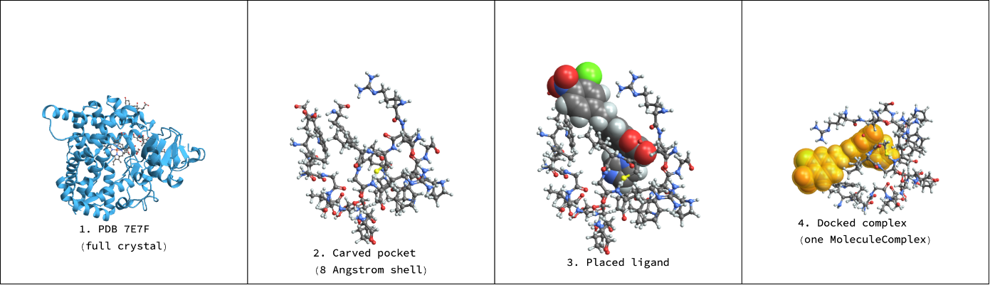
Overview of the docking process. The simulation is prepared by importing the 7E7F crystal structure with the inhibitor metyrapone. The step-by-step transformation is shown above: (1) isolating the target protein, (2) defining the 8 Å binding pocket shell around the heme porphyrin ring, (3) placing and optimizing the ligand near the active site, and (4) assembling the final unified molecule complex.
Initializing the Environment
Initializing the Environment
I use the MoleculeComplex paclet, developed by Dr. Robert Nachbar and available in Wolfram’s paclet repository. This adds the MoleculeComplex, MoleculeComplexOptimizeGeometry, and MoleculeComplexEnergy functions on top of the built-in Molecule framework, and lets us treat a ligand plus a set of protein-pocket fragments as one multi-component system that can be optimized and scored for intermolecular energies using the MMFF94 forcefield.
In[]:=
PacletInstall["RobertNachbar/MoleculeComplex"]Needs["RobertNachbar`MoleculeComplex`"]
Out[]=
PacletObject

Visualizing the Ligand-Protein Complex
Visualizing the Ligand-Protein Complex
First, I import the CYP11B1 crystal structure 7E7F (human 11-β-hydroxylase co-crystallized with metyrapone at 1.40 Angstrom) from the Protein Data Bank. This structure provides us an experimentally resolved model of the CYP11B1 active site and its surrounding catalytic environment. BioMolecule returns the full assembly, including protein (chain A), heme (chain B), and the crystallographic ligand, metyrapone, bound to the protein.
In[]:=
cysPDB=BioMolecule[ExternalIdentifier["PDBStructureID","7E7F"]]
Out[]=
BioMolecule

Plot the entire assembly with BioMoleculePlot3D (protein drawn as a cartoon ribbon, hetero-atoms as sticks):
In[]:=
BioMoleculePlot3D[cysPDB]
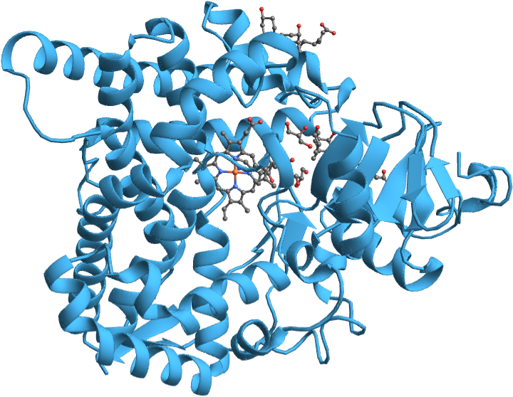
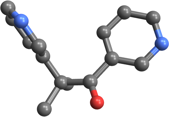
The molecular structure contains water molecules surrounding or bound to the protein. The assembly can be decomposed by selecting for specific chains that are not water molecules or non-polymers. Identifying each of them lets us inspect and later re-use them independently if needed. To isolate the metyrapone ligand, chain C is selected.
In[]:=
metyraponeLigand=BioMolecule[cysPDB-><|"Chains"->{"C"}|>]
Out[]=
BioMolecule

Plot the metyrapone ligand:
In[]:=
BioMoleculePlot3D[metyraponeLigand]
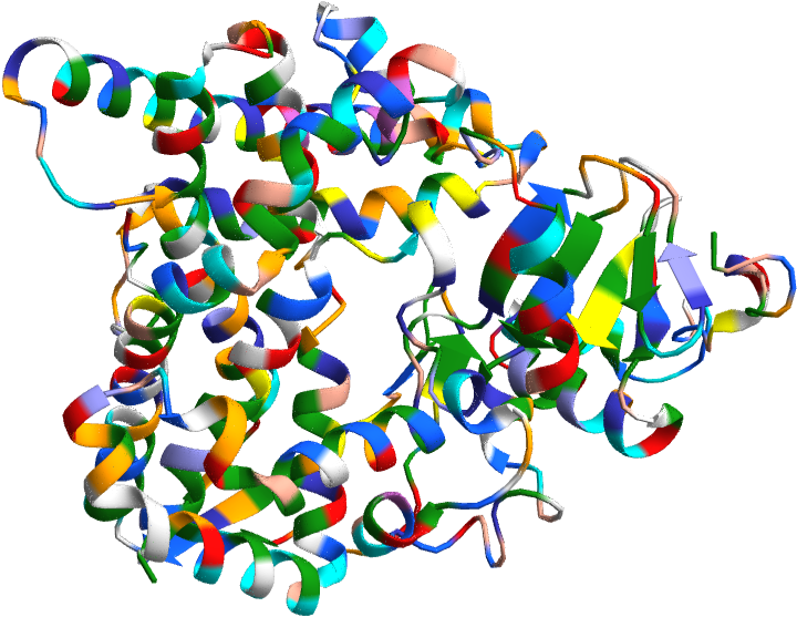
Isolate the protein without the heme (chain A):
In[]:=
cysPDBEnzymeOnly=BioMolecule[cysPDB-><|"Chains"->{"A"}|>]
Out[]=
BioMolecule
Plot the enzyme with its residues as color rules:
In[]:=
BioMoleculePlot3D[cysPDBEnzymeOnly,ColorRules->"Residues"]
Isolate the protein with heme (chains A and B):
In[]:=
cysPDBEnzymeWithHeme=BioMolecule[cysPDB-><|"Chains"->{"A","B"}|>]
Out[]=
BioMolecule
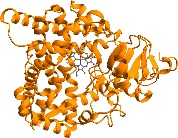
Plot the protein with heme, highlighting the protein in orange:
In[]:=
BioMoleculePlot3D[cysPDBEnzymeWithHeme,ColorRules->{_->Orange}]
Visualizing Metyrapone-Protein Interaction Through the Heme
Visualizing Metyrapone-Protein Interaction Through the Heme
11-β-hydroxylase encoded by CYP11B1 is a mitochondrial cytochrome P450 enzyme. These enzymes are a superfamily of heme-containing mono-oxygenases responsible for oxidizing steroids, fatty acids, and xenobiotics in mammals, along with other synthesis functions in plants and bacteria. Cytochrome P450 enzymes use heme to oxidize their substrates for binding, consuming protons from NADH or NADPH to split the oxygen so that a single atom can be added to the substrate (InterPro, n.d.). The heme is the catalytic cofactor shared by all cytochrome P450 enzymes: a flat iron-porphyrin ring (a separate component, chain B of 7E7F) with a single iron atom at its center, where the interaction between the enzyme and active site occurs. The heme is thus a point of focus among the rest of the crystallographic material.
Zooming into the catalytic center, one face of the heme iron is held by a protein cysteine (Cys450, the proximal ligand), while the opposite or distal face points into an open cavity. That cavity is the active site, where both the natural substrate of the protein and any inhibitor must bind. By placing its own coordinating nitrogen on the iron, also known as a type-II spectral shift, the inhibitor occupies the site required by the substrate’s oxygen chemistry (Mukai et al., 2021).
Zooming into the catalytic center, one face of the heme iron is held by a protein cysteine (Cys450, the proximal ligand), while the opposite or distal face points into an open cavity. That cavity is the active site, where both the natural substrate of the protein and any inhibitor must bind. By placing its own coordinating nitrogen on the iron, also known as a type-II spectral shift, the inhibitor occupies the site required by the substrate’s oxygen chemistry (Mukai et al., 2021).
ShowMoleculePlot3DMolecule[BioMolecule[cysPDB-><|"Chains"->{"B"}|>]],,MoleculePlot3D[Molecule[BioMolecule[cysPDB-><|"Chains"->{"C"}|>]]],
Above is a visualization of the heme-metyrapone coordination in the active site. Within this complex, one of its ring nitrogen atoms (in blue) points at the iron’s open distal face and “coordinates” it. The nitrogen lone pair donates into the iron, forming a bond roughly 2.09 Angstrom long that blocks the site. Binding other inhibitors to this ring relies on the coordinating nitrogen interacting with the iron.
Plot the molecular structure of metyrapone:
Each of the two coordinating nitrogens (blue) has exactly two bonds, a single bond and a double bond, making them easily identifiable programmatically.
Constructing the Inhibitor Library
Constructing the Inhibitor Library
The five inhibitor candidates I analyze share one scaffold: a coumarin molecule bearing an imidazolylmethyl ‘warhead’, a term in medicinal chemistry for the reactive end of a drug. In this case, the warhead concerns the imidazole ring, and specifically its coordinating nitrogen. This nitrogen anchors the molecule at the catalytic center, binding the heme iron. The remainder of the scaffold contributes to pocket complementarity and modulates the electron density at the coordinating atom. Moreover, each inhibitor contains a benzyloxy tail carrying a para-nitro group plus a variable ortho substituent.
I store the five inhibitors in a name-keyed association so that every downstream step can be indexed by ligand name rather than list position.
I store the five inhibitors in a name-keyed association so that every downstream step can be indexed by ligand name rather than list position.
Import the five inhibitors through their derived SMILES strings:
Plot their 2D structures in a grid:
All of the inhibitors D1 through D5 differ only in their ortho substituent. D1 has Chlorine (Cl), D2 has Bromine (Br), D3 has Fluorine (F), D4 has a methyl group (CH3), and D5 has a hydroxide group (OH). One change at a time on the southern ring systematically varies steric size and electronics.
Plot their 3D structures:
Conformer Generation and Molecular Flexibility
Conformer Generation and Molecular Flexibility
Before a ligand can be docked, one has to decide which of its many possible conformations to dock depending on its torsional freedom. Because such a molecule can rotate about its single bonds, it is best described not as a single fixed structure but as a thermally accessible ensemble of conformers separated by low torsional barriers. This conformational freedom determines the entropic cost for a ligand to associate with the target and how readily the molecule can adapt to the contours of the active site. Conformer generation samples that ensemble prior to energy minimization. Taking on the order of thirty geometries or conformers approximates the accessible states and guards against proceeding into docking with a single, possibly strained or unrepresentative conformation.
MoleculeModify allows for generation of conformers through built-in torsion-driving functionality. Specifically, the GenerateConformers parameters samples a diverse set of low-strain 3D geometries for a given molecule. The generator is mapped over the whole association at once, so allConformers is again name-keyed (D1 -> {30 conformers}, ...). Thirty conformers per ligand allows for thorough coverage of the conformational space.
MoleculeModify allows for generation of conformers through built-in torsion-driving functionality. Specifically, the GenerateConformers parameters samples a diverse set of low-strain 3D geometries for a given molecule. The generator is mapped over the whole association at once, so allConformers is again name-keyed (D1 -> {30 conformers}, ...). Thirty conformers per ligand allows for thorough coverage of the conformational space.
At times, GenerateConformers may not fully generate conformers that are all different from each other. I determine whether conformer generation occurred successfully by superimposing the conformers on top of each other and visually comparing them for differences in orientation.
Inspect one ligand's conformer ensemble, all overlaid:
Energy Minimization
Energy Minimization
The geometries are evaluated with a molecular-mechanics force field (MMFF94), an empirical potential that represents a molecule as a network of classical terms, including harmonic bond and angle restraints, torsional profiles, and nonbonded van der Waals and electrostatic contributions, and is parameterized to reproduce experimental quantum-chemical data. As it does not concern solving the electronic Schrödinger equation, it achieves remarkable speed with molecule relaxation but is blind to explicit electronic structure. As such, it carries no parameters for transition-metal centers like the heme iron.
Raw sampled conformers sit at arbitrary points on the energy surface, and each one is relaxed to its nearest local minimum on the MMFF94 force field. The inner map runs EnergyMinimizeAtomCoordinates over each conformer of one ligand; the outer map applies that to every ligand, so minimizedConfs preserves the name-keyed structure of the original conformer set.
View the conformers for D1:
Force-field minimization sometimes drives several distinct starting conformers into the same final geometry. To fully validate the conformer set, removeDuplicates collapses nearly identical structures if they have an an element-wise difference less than 0.01 Angstrom.
DistanceMatrix gives the matrix of distances between pairs of atoms for a given molecule. In this function, I define a condition that a conformer molecule is the same as another if the difference between one atom-to-atom pair distance and another is greater than 0.01 Angstrom. DeleteDuplicates takes in our condition as a testing parameter to delete the nearly identical conformers. However, it is important to note that there is no common distance threshold for identical conformers. Thus, this filter may not cover every possible similarity.
Apply DistanceMatrix to the magnitude of the atom coordinates and compute the absolute maximum values of the difference, deleting the duplicates based on the condition:
Apply removeDuplicates to the minimized conformers to filter them into a list of unique conformers:
Only the thermally relevant conformers are kept. The built-in force field used for energy evaluation is the Merck Molecular Force Field (MMFF94s), accessed via the “MMFFsEnergy” property. curateConformers removes units from each MMFF energy, finds that ligand's global minimum, keeps everything within a 3 kcal/mol window above it, and returns at most the five conformers with the lowest energies in the set.
Construct pairs of conformers and their energies, and then select the smallest-energy conformers within a window of minEnergy + 3:
Apply curateConformers to the list of unique conformers, filtering it further into a list of curated conformers:
Verify how many of the conformers were kept in the process by comparing the length of the lists:
Plot the values across all three lists in a dataset:
For clarity, I verify that the curated conformers actually have the lowest energies by comparing them to the expected lowest energies from the total list of conformers for D1.
Obtain the energies of curatedConfs from D1 and store into curatedEnergiesD1:
Obtain the energies of all conformers from D1 and store into allEnergiesD1:
Take the five conformers with the smallest energies from allEnergiesD1 and store into lowestExpectedEnergiesD1:
Display the dataset as a comparison:
The two lists of energies seen here are identical, meaning that the curation process worked as expected.
Active-Site Pocket Preparation
Active-Site Pocket Preparation
As my environment does not have the processing power necessary to dock small molecules on the entire protein, the protein is trimmed down to a smaller region, the binding pocket. Specifically, the pocket is carved from the original protein around two fixed points, or anchors that mark the catalytic center: the heme iron (atom FE) and metyrapone’s coordinating nitrogen (atom N14). As these two atoms define where catalysis happens, any residue near them is part of the functional binding site.
First, I obtain and flatten every atom's label and coordinate into a table so I can find named atoms by string before verifying the distance between the coordinating nitrogen and heme iron atom.
Obtain the atom labels by filtering for strings:
Obtain the coordinates for all atoms in the entire protein complex by computing the magnitude of each QuantityMatrix, filtering for numerical values:
Construct an atom table with the labels and coordinates:
Extract the two anchor coordinates by atom label: the heme iron (FE) and the metyrapone coordinating nitrogen (N14):
Compute the Euclidean distance between N14 and FE, which we expect to be roughly 2.09 Angstroms:
I now cut the binding pocket out of the full protein, keeping only residues that line the active site. I define a residue as kept if any of its heavy atoms falls within 8 Angstrom of either anchor (the heme iron or the metyrapone coordinating nitrogen).
I do this in a five-step process:
I do this in a five-step process:
◼
Locate the anchor coordinates
◼
Set an 8 Angstrom cutoff by testing each residue for whether any of their atoms are within this range
◼
Associate individual atoms with their residues to trim the protein by residue
◼
Delete the farthest atoms by mapping the residue cutoff test onto them
◼
Split the remaining structures into fragments of the binding pocket to assemble into a complex
In the process, the binding site will include the full active site where each inhibitor interacts with the enzyme and only complete residues within this radius to create an accurate model for the pocket.
Collect the anchor coordinates from before:
Set the cutoff and test (nearRef):
Remember that the binding pocket is carved out of the enzyme only (the object below), as this will ultimately be used to form our complexes.
Build the protein as one Molecule and read its per-atom coordinates (atomCoords):
atomCoordsFlat is a flat list of all atom coordinates in the protein, which will be filtered for the coordinates of the binding pocket atoms:
Group heavy-atom coordinates by residue (chain A), so each residue is a list of its atom positions:
Mark each residue True if any of its atoms is inside the cutoff:
Tag every atom (represented by their coordinates) with the residue number before flattening the coordinates:
Preview this list:
Create a Nearest function that takes in an atom coordinate pair as input and outputs the residue associated:
Map this function onto the list of atom coordinates and output the number of the nearest residue for each atom:
Preview this list:
keepAtomTest marks whether the atoms should be kept by mapping keepResidueTest onto their residue numbers:
A preview of what this list looks like:
Collect the indices to delete (deleteIndex) :
The number of residues kept intact can be counted by looking at the number of True values in keepResidueTest and the total number of residues by the length of the list.
Similarly, the number of True values in keepAtomTest indicates the number of atoms kept, and the total length of the list indicates the total number of protein atoms.
The binding pocket is highlighted here in orange and the heme iron position as a red sphere. The highlighted pocket is defined by keepIndex, the list of atoms our protein is trimmed down to.
Plot the binding pocket, coloring the atoms indexed by keepIndex orange:
Keeping every residue with an atom within 8 Angstrom of either anchor yields a shell of 25 residues, the wall of the active-site cavity. This is small enough to model explicitly and complete enough for bounding a ligand using MoleculeComplex. Note these 25 residues are not all separate. Where several kept residues are consecutive in the protein chain, they remain peptide-bonded. The next step groups the 25 residues into a smaller number of covalently connected fragments.
Delete the farthest atoms, then restore explicit hydrogens so each fragment is a chemically complete piece:
The trimmed structure is split into covalently connected fragments. The 25 kept residues collapse into 9 connected pieces (395 atoms total). All five inhibitors will later be placed into this identical pocket.
Connect the trimmed components to form the building blocks for the binding pocket dock (pocketFragments):
We can look at the carved pocket on its own, and as an assembled MoleculeComplex:
Assembled Binding Pocket
Assembled Binding Pocket
Assembling the nine fragments into a single MoleculeComplex highlights for us the active site and receptor every inhibitor is docked against. The most important aspect of this is the heme porphyrin ring (colored in orange).
Carved CYP11B1 active-site pocket with 25 residues collapsed into 9 covalently connected fragments (395 atoms), assembled as one MoleculeComplex. This shared receptor is reused for all five inhibitors.
Docking Implementation
Docking Implementation
Ligand Placement and Warhead Identification
Ligand Placement and Warhead Identification
I made two functions to place the ligand deterministically closer to the active site. The goal here is to translate each ligand so that its imidazole coordinating nitrogen lands exactly on the metyrapone nitrogen (mytNXYZ), reproducing the iron-coordination geometry present in the original binding interaction. This will allow alignment of the small molecule’s geometry so that it better fits into the binding pocket during optimization.
findCoordN locates the coordinating nitrogen in the ligand, the aromatic imidazole N bonded to exactly two heavy atoms. This nitrogen is the coordinating atom that binds to the heme iron in the CYP active site during the process of inhibition. placeLigand uses this information to place the ligand by aligning the nitrogen in the ligand with the metyrapone nitrogen.
findCoordN locates the coordinating nitrogen in the ligand, the aromatic imidazole N bonded to exactly two heavy atoms. This nitrogen is the coordinating atom that binds to the heme iron in the CYP active site during the process of inhibition. placeLigand uses this information to place the ligand by aligning the nitrogen in the ligand with the metyrapone nitrogen.
Store the symbols of the atoms and the bonds in variables, then select for the first nitrogen that shares two bonds using MemberQ, returning its index:
Highlight the coordinating nitrogen atom in orange (on the five ring):
As seen here, findCoordN correctly identifies the coordinating nitrogen for D1’s first conformer.
Rigidly translate every atom of the conformer by calculating the vector that moves that nitrogen onto mytNXYZ with findCoordN and applying this quantity to the coordinates:
Complex Assembly and Optimization
Complex Assembly and Optimization
With the ligand placed, it is assembled with the pocket fragments into a single MoleculeComplex. Prepend puts the ligand first (component 1), so it can be addressed as component 1 in the highlighting and atom-count calls below.
Take the lowest-energy curated D1 conformer, make its hydrogens explicit, and place it in the pocket:
Assemble the ligand-and-pocket complex and view it entirely as spacefilling to better visualize the geometry (ligand highlighted):
Though the ligand has been placed into the binding site, the geometry has not been optimized to find the lowest possible energy of the complex. MoleculeComplexOptimizeGeometry runs a local MMFF94 energy minimization over the complex’s atomic coordinates, relaxing the assembly to a nearby force-field minimum and minimizing the energy of the complex.
Optimize the complex geometry, using Quiet to suppress harmless warnings:
Re-plot the relaxed pose of the complex:
Compute the raw complex energies, before and after optimization:
As expected, the energy of the complex decreases drastically after optimization. A visual is provided to better understand the comparison.
Plot both the placed and optimized versions here:
Ligand Placement and Complex Assembly
Ligand Placement and Complex Assembly
With the pocket carved and placement functions defined, the pipeline is compiled into a set of three functions: placeAndAssemble, coordDist, and pocketAtoms. For every ligand, the lowest-energy curated conformer is translated so the imidazole nitrogen aligns with the metyrapone-N anchor (~2.09 Angstrom from the heme iron), added with explicit hydrogens, joined with the pocket fragments into a single MoleculeComplex, and relaxed on MMFF94. MoleculeComplexOptimizeGeometry is a local minimizer, which is why the ligand must be positioned in the coordinating pose first.
placeAndAssemble places a conformer near the binding site using the placeLigand function, adds hydrogens by making them explicit, builds the molecule complex, and returns the optimized complex based on the process defined earlier. Essentially, this function consolidates both of the functions for ligand placement and complex formation.
Using the coordinate finder (coordN), coordDist computes the distance between the imidazole nitrogen atom and heme iron atom in order to verify that the placement of the ligand reproduces the ~2.09 Angstrom coordination geometry.
Locate the coordinating nitrogen on each placed ligand and finds its Euclidean distance to the iron:
Use the Nearest function to count and filter how many ligand heavy atoms sit within 4 Angstrom of a pocket atom (cutoff):
To demonstrate these functions, D1’s lowest-energy conformer is once again assembled and rendered, and the ligand (shown as spacefilling) is highlighted against the pocket residues:
Using the functions defined earlier, the placement geometry and pocket fit (in number of atoms) for D1 is verified below.
Measure the Fe/N coordinate distance:
Measure the number of heavy atoms of the ligand within 4 Angstroms of the binding site:
Assemble complexes with the curated conformers from each of the inhibitors D1-D5 and create an association with them:
For efficiency, previously optimized complexes with all of the conformers can be obtained by pulling their information from the cloud:
Plot the complexes with D1’s conformers in a grid:
As seen here, the conformations change their binding positions, which is expected to result in differing values for complex energies.
Computing Energies of Complexes
Computing Energies of Complexes
Having assembled each curated conformer into the pocket, the MMFF94 energy of every optimized complex can be read. All conformers of one ligand share the same atoms and the same pocket, and so these energies are comparable within a ligand. Specifically, these energies can be used to identify which placed conformer relaxes to the most stable bound arrangement.
Create a function which computes the energy for each conformer complex:
Use computeEnergies to compute the energies of each conformer complex, creating an association with all of them:
Structure-Function Analysis
Structure-Function Analysis
Measuring Conformational Sensitivity
Measuring Conformational Sensitivity
The differences between the conformer energies and a baseline energy, which is defined here as the minimum-energy conformer, can be readily measured. This allows us to obtain a sense of the variability between conformers and therefore the sensitivity of conformational changes across all inhibitors. Essentially, the conformer that forms the lowest-energy complex is the conformer that will bind to the protein most effectively out of the five. Knowing the lowest-energy conformer allows us to design analogs or versions that adopt this conformation more often.
I create a multivariable table to better contain and compare our results across the five ligands and their conformers. For each conformer, the chart below identifies the ligand it corresponds to, its number, the energy of its complex, and the ΔE between the conformer’s energy and that of the best-scoring conformer, the lowest energy value for the ligand.
Use a pure function that takes the ligand and curatedEnergies as input and returns a list indexing the number and computing the energy difference for each conformer:
Construct a nested association containing values for E and ΔE, grouped by conformer number:
Extract unique ligand names to build the header columns dynamically :
Generate the table rows by cleanly extracting the formatted values with a Table:
Create headers to label the energy values on the horizontal table:
Combine and render the final Grid:
The energies tabulated here invite a natural comparison across the five ligands, and it is important to recognize why that comparison is not valid. A force-field energy is defined only relative to an internal, molecule-specific reference. As such, its absolute value has no physical meaning and is not conserved across chemically distinct species. Differences taken within a single ligand, however, are interpretable, as these values rank that ligand’s own conformers by relative stability. On the other hand, differences taken across ligands are not interpretable since the zero of each molecule is set independently. Accordingly, every energy in this study is read and compared down a single ligand’s column, while the only comparisons that can be drawn across the D1–D5 series are purely geometric.
Plotting the conformer’s ΔE values on a ListPlot allows us to gain a visual understanding of the variability across ligands in terms of their conformer energies. Here, I define a separate function (calcStability) that computes the energy differences listed previously, and use this to compute raw values for the energy differences which are then mapped onto the plot.
Compute the difference between each energy and the lowest:
Map the calcStability function onto the values for curatedEnergies by indexing them by key:
Compute the energy differences in a list for each ligand and plot them by conformer:
Using the functions defined earlier, I mainly compute the number of atoms of each inhibitor coming in close proximity with the binding pocket. Here, I create a table summarizing the conformer line for each ligand, their “best” or most minimized complex energy, the measured bond length between the nitrogen atom and heme iron of the placed conformer, the number of pocket atoms in contact, and whether the ligand’s conformer series contains an outlier. As MMFF energies are not applicable to Fe···N interactions, no coordination is imposed onto the forcefield and scored.
Store the ligand number, number of conformers, best-scoring energy, Fe···N distance, number of atoms in contact, and whether the energy is an outlier using the condition that it exceeds 500 kcal/mol:
Plot the table with these values:
Here, all conformers and ligands show identical values for bond distance between the iron and nitrogen atoms due to intentional placement. The differences between the best energies of the complexes are relatively modest, suggesting that differences in chemical structure between inhibitors have less of an impact on the complex formations.
Structural Comparison: Comparing Binding Modes
Structural Comparison: Comparing Binding Modes
More qualitative conclusions can be drawn by comparing this essay’s docking approach to that of our reference, El Yaqoubi et al. In our evaluation, each molecule D1–D5 was seated on the distal side of the heme by anchoring its coordinating imidazole nitrogen to the crystallographic metyrapone-nitrogen site, so that every pose reproduces the axial heme-coordination geometry. The methodological basis and limits of this placement are discussed under the Limitations and Future Directions section. In contrast, the reference paper scored each pose on a fingerprint of peripheral contacts, two to five per molecule and spanning residues including Arg110, Arg384, Arg404, Arg412, Arg454, Glu383, Leu113, Leu451, Cys450, and Trp428, without requiring any ligand atom to occupy the sixth coordination position of the iron.
Thus, the two processes favor different binding modes. This contrast is seen clearly for D3, the leading inhibitor of the series according to the reference. Our placement directs D3 toward axial the coordination that defines traditional inhibition of cytochrome P450 enzymes, the same mode by which the inhibitor fadrozole binds to the heme iron in PDB 6M7X, which involves the same enzyme with a different ligand. El Yaqoubi et al. employs an unconstrained search that directs D3’s coordinating imidazole nitrogen toward the guanidinium of Arg404 (a pi-cation contact at 3.26 Å), with a pi-H contact to Leu113 at 4.69 Å enclosing the scaffold among hydrophobic residues.
Thus, the two processes favor different binding modes. This contrast is seen clearly for D3, the leading inhibitor of the series according to the reference. Our placement directs D3 toward axial the coordination that defines traditional inhibition of cytochrome P450 enzymes, the same mode by which the inhibitor fadrozole binds to the heme iron in PDB 6M7X, which involves the same enzyme with a different ligand. El Yaqoubi et al. employs an unconstrained search that directs D3’s coordinating imidazole nitrogen toward the guanidinium of Arg404 (a pi-cation contact at 3.26 Å), with a pi-H contact to Leu113 at 4.69 Å enclosing the scaffold among hydrophobic residues.
2D interaction diagram of compound D3 docked within the active site of the 6M7X protein (reproduced from El Yaqoubi et al., 2026, Scientific African, under CC BY 4.0).
Binding-mode comparison for D3. (Left) Reported docking pose of compound D3 with 6M7X binding pocket (reproduced from El Yaqoubi et al., 2026, Scientific African, under CC BY 4.0): the imidazole nitrogen is directed toward Arg404, with the scaffold enclosed by hydrophobic residues. (Right) This work: the same imidazole nitrogen is placed axially to the heme iron.
These two poses are mutually exclusive in geometry. The coordinating nitrogen is an sp2-hybridized, pyridine-type nitrogen whose lone pair can be donated in only one direction. In El Yaqoubi et al.’s binding pose, that lone pair is committed to the electrostatic contact with Arg404, leaving it pointed away from the iron. Therefore, it cannot satisfy the axial coordination to the heme that defines this inhibitor class. The question of which pose is more physically meaningful thus reduces to whether the coordinating nitrogen engages the catalytic metal or a pocket residue surrounding it. Our geometric model attempts to answer this question by construction, while their paper does so via spatially unconstrained scoring.
Exploring Shape Similarity in Molecular Docking
Exploring Shape Similarity in Molecular Docking
Shape similarity scoring often complements the process of docking. While docking simulates movement of molecules and scores them within a target’s binding site, shape similarity assesses how closely a candidate’s ligand, including its steric properties and pharmacophores, matches the 3D shape or volume of the target protein (Hawkins et al., 2007). Modern methods such as ROCS have been used to find novel molecular scaffolds that are ideal in shape for binding using Gaussian functions (OpenEyes, n.d.).
To explore shape similarity, I utilize Gaussian meshes of the protein and molecules to evaluate whether the shape of the ligand's molecular surface matches the shape of the protein it binds to. Effective binders should be shape-complementary, or convex where the protein or pocket is concave, and curving on the same length scale. To measure this, I represent each surface as a set of small local patches of points and reduce every patch to a few differential-geometry numbers (a surface normal and its curvatures). Those per-patch numbers are correlated between the protein and ligand to find shape similarities. Equations for all calculations and scores can be found in Supplemental Information. Two objects from the docking pipeline are reused unchanged but redefined as new variables: cysPDBEnzymeShape, the entire enzyme, and d1ConformerShape, the placed D1 conformer.
To explore shape similarity, I utilize Gaussian meshes of the protein and molecules to evaluate whether the shape of the ligand's molecular surface matches the shape of the protein it binds to. Effective binders should be shape-complementary, or convex where the protein or pocket is concave, and curving on the same length scale. To measure this, I represent each surface as a set of small local patches of points and reduce every patch to a few differential-geometry numbers (a surface normal and its curvatures). Those per-patch numbers are correlated between the protein and ligand to find shape similarities. Equations for all calculations and scores can be found in Supplemental Information. Two objects from the docking pipeline are reused unchanged but redefined as new variables: cysPDBEnzymeShape, the entire enzyme, and d1ConformerShape, the placed D1 conformer.
Mesh Creation
Mesh Creation
Define the protein and ligand objects for creating meshes:
I first mesh the entire enzyme (protMesh). Rendering cysProteinMesh shows the full protein surface: a large, closed body whose exterior is mostly far from the binding cleft, which sits as a dimple in it.
As a proof-of-concept, I study the shape similarity between the protein and conformer 1 of D1. protMesh and d1Conf1Mesh are the two surfaces used for the complementarity comparison from here on.
Build the protein surface and the ligand surface with identical settings so the two are directly comparable:
Graph the two surfaces:
MeshCoordinates gives a mesh's vertex coordinates, while RegionCentroid gives its center of mass. I obtain both for each surface, because the sampling step needs the point clouds and the normal-orientation step requires the centroids. I introduce four objects: protMeshPts, d1Conf1MeshPts, comProtein, and comd1Conf1 for the mesh coordinates and centers of mass.
Store the mesh coordinates for the protein and ligand meshes {x, y, z}:
Calculate and store the centroids for the meshes:
Compare the number of vertices of each surface in a table:
Computing Normals for Protein and Ligand Surfaces
Computing Normals for Protein and Ligand Surfaces
For reference later, I define the per-vertex outward normal vectors straight from each mesh, in order of the mesh coordinates. EstimatedPointNormals least-squares-fits a plane to each vertex’s neighbors.
Use EstimatedPointNormals to calculate normal vectors from all of the mesh coordinates for the protein and ligand:
Sampling Points on the Protein and Ligand Meshes for Centers
Sampling Points on the Protein and Ligand Meshes for Centers
To describe a surface locally, we need a set of sample centers spread evenly over it. I used Farthest-Point Sampling (FPS), which samples the mesh's own vertices by starting from one vertex and repeatedly adding whichever vertex is farthest from everything chosen so far. The algorithm keeps, for every vertex, its distance to the nearest already-chosen center, so the selection spreads out over the whole surface, including the concavities, instead of clustering. It returns the indices of the chosen vertices. farthestPoints is the function that encodes this algorithm.
Input the mesh coordinates, start with i as the largest distance from the center, compute the Euclidean distances between new points and already-sampled centers, and append the points with the minimum-maximum distances from the sampled points (indexed in state with i) to an empty list, returning a list of coordinates for the centers of length nCenters:
Now, I sample both surfaces for points. The protein is much larger than the ligand, so I intentionally define a greater number of centers.
Set the number of centers for the protein (400 centers) and ligand (40 centers):
Apply farthestPoints to the mesh coordinates with the numbers of centers and store the equally spaced points into variables, one for each surface:
To check that the sampling occurred as intended, I overlay the chosen center vertices on each surface. Satisfactory coverage looks like points spread roughly uniformly, reaching into the concave regions rather than bunching on one face. If they clustered, the descriptor set would be biased toward whatever part of the surface was over-sampled. The pocket (red) carries more, coarser centers, while the ligand (blue) carries fewer, finer ones.
Plot the two meshes with their centers as points in a GraphicsRow:
Creating Patches From Surface Centers
Creating Patches From Surface Centers
A patch of points is defined as a small, roughly disc-shaped cap of the surface, small enough that one surface normal vector and one pair of curvatures can describe it well. patchesFromCenters creates a patch around each surface center that will be later used to describe parts of the surface.
Define the radii of the patches for the protein and ligand:
Given a point, return the indices of nearby vertices sorted by distance and then obtain all vertices within the radius r of a center in order of distance:
Apply patchesFromCenters to create the patches for the protein and ligand:
Create a grid containing the number of patches and the median number of points for each patch:
We can plot a single center with its patch on the surface on the protein to make it tangible. I highlight the vertices of one pocket patch by flattening a chosen element of patchesProt and indexing from this list.
Plot the points of one patch by flattening and indexing from patchesPlot:
Obtaining Surface Descriptors from Patches
Obtaining Surface Descriptors from Patches
Quantifying shape similarity requires compiling features, or descriptors for each surface patch. The function patchDescriptorsBuiltin reduces one patch to its descriptor, consisting of its center coordinates, surface normal vector coordinates, principal, mean and Gaussian curvature values, shapeIndex, curvedness, and number of points.
First, I obtain the surface normals from the values calculated earlier. However, this local fit is unable to tell concavity from convexity, so I flip its sign so it points away from the surface’s centroid (i.e. outward). Second, Wolfram allows me to calculate the curvature. On a mesh, the RegionMaxCurvature, RegionMinCurvature, RegionMeanCurvature, and RegionGaussianCurvature functions are discrete, per-vertex quantities. So, I evaluate them at the patch's vertex index, obtained from farthestPoints. The AllTrue test filters out any patch whose curvature still fails to reduce to a number. From the two principal curvature values k1 (max) and k2 (min), I form two scale-aware summaries: the shape index (the type of local shape: -1 cup, 0 saddle, +1 dome) and the curvedness, or curv >= 0 (how sharply it curves).
First, I obtain the surface normals from the values calculated earlier. However, this local fit is unable to tell concavity from convexity, so I flip its sign so it points away from the surface’s centroid (i.e. outward). Second, Wolfram allows me to calculate the curvature. On a mesh, the RegionMaxCurvature, RegionMinCurvature, RegionMeanCurvature, and RegionGaussianCurvature functions are discrete, per-vertex quantities. So, I evaluate them at the patch's vertex index, obtained from farthestPoints. The AllTrue test filters out any patch whose curvature still fails to reduce to a number. From the two principal curvature values k1 (max) and k2 (min), I form two scale-aware summaries: the shape index (the type of local shape: -1 cup, 0 saddle, +1 dome) and the curvedness, or curv >= 0 (how sharply it curves).
Before calculating the shape index, I calibrate its sign, represented by the variable siSign. RegionMaxCurvature/RegionMinCurvature orients curvature to the mesh's own normal. For a MoleculeMesh isosurface, that normal can point inward. I measure the sign on an object whose answer is known: a solid sphere seen from outside is convex everywhere,so its shape index must be+1. I compute the mean shape index on a discrete sphere with siSign temporarily as 1. If this value is negative, the convention is flipped and I set siSign = -1, otherwise positive 1. Every descriptor computed afterwards picks up this siSign automatically.
Define the mesh coordinates and centroids for a sphere, computing the shape index and changing siSign depending on its sign:
Given the mesh, its coordinates, normal vectors, center of mass, and information about the specific patch, I create the descriptors for that patch.
Compute the normals with the curvature functions and curvedness and shape index formulae, then store them into an association of descriptors:
I run the same descriptor function on both surfaces so the two sets of numbers (proteinDesc and d1Conf1Desc) are directly comparable.
Use MapThread to pair each center index with its patch and create the protein descriptor, applying DeleteCases to remove any patch descriptors that returned Nothing:
Similarly compute the ligand descriptor:
View one of the protein descriptors:
With the descriptors computed, I can now draw the two geometric quantities they carry. First, the normals are drawn here as an outward arrow at each pocket-patch center. They are expected to extend outward from the surface as a verification that that the sign-flip against the centroid worked.
Plot the surface normal vectors as red arrows on the protein and ligand centers:
Second, I plot the shape index as colored points painted onto the surface. I color each center by its shapeIndex through a diverging color scale: one end for cups (concave, -1), the other for domes (convex, +1), and the middle for saddles. This is the most informative descriptor for complementarity, as a concave pocket should align with a convex ligand dome. Visualizing this quantity on the surface directly informs us where the pocket is bowl-like versus protruding outwards.
Plot the centers with temperature colors corresponding to the shape index (cups are categorized blue, and domes are categorized red):
Define the columns:
Create a function that creates rows with the descriptor values by keying into the association:
Make the rows from the protein descriptors by using MapIndexed, which retrieves the index of each element as the patch number (ID) and then appends the remaining descriptor values for that patch:
Repeat this for the ligands:
Construct two tables with the first ten rows, one for the ligands and another for the protein descriptors:
The tables above display descriptors for the first ten patches mapped onto the surfaces.
Quantifying Shape Similarity of Patches Using Descriptors
Quantifying Shape Similarity of Patches Using Descriptors
Encode the equations into a function that takes in a patch and ligand descriptor and outputs the score:
Now, I score every pocket-patch/ligand-patch pair and keep the ranking in a variable (allPairScores) to retrieve later.
Call compScore directly inside the Table, having each row of allPairScores of the form {pocket index i, ligand index j, score}:
Pull the 15 lowest scores (the 15 most complementary pairs) as {i, j} using TakeSmallestBy:
Take the single best pair from the list of pairs ranked by their score (bestPairsRanked):
Preview the rankings in a table:
To better visualize what the complementarity score checks for, I plot the best ranked pair of pocket and ligand patches. I retrieve the actual points of the best ranking pocket patch and the best ranking ligand patch, then recenter each of them on its own centroid so the two caps sit at a common origin and can be compared side by side.
Retrieve the points of the best patch on the protein and store in a variable:
Similarly retrieve the points of the best patch on the ligand:
Position the points near the centroid:
Plot the two patches in red to compare side-by-side:
In the spirit of the pocket formation earlier, the patch can also be assessed to see whether it lies in the binding pocket and if not, how far it lies away from the heme iron near the active site.
Retrieve the centroid of the best ranked patch by key:
Calculate the Euclidean distance between the centroid and iron (with coordinates feXYZ):
Create a table summarizing the coordinates and analysis:
It would help to visualize the patches spatially with the surfaces on which they were originally mapped. I overlay them onto the meshes here (highlighted in red), making it easier to observe that the protein patch is quite far from the inner binding pocket.
Define a color for our patch (red):
Store the protein with the overlaid patch as a Show object:
Store the ligand with the overlaid patch as a Show object:
Display both Show objects here as a row:
Analysis of Protein-Ligand Intrinsic Fit Using RMSD
Analysis of Protein-Ligand Intrinsic Fit Using RMSD
The shape index and normals answer the question of whether two patches fit extrinsically, but another crucial question to ask is whether the protein and ligands patches fit intrinsically. To do this, I compute a distance signature that does not depend on how either patch is rotated or where it sits in space. Specifically, I reduce each patch to the sorted list of distances between its own points. As those internal distances do not change with rotation or transformation, two patches with the same signature have the same shape. distSignature creates this geometrical fingerprint.
Pull the actual coordinates of the patch points (P) and compute the Euclidean distances between all of them using Table, sorting them into the same list:
Calculate a distance signature by taking four points in a patch on the protein, noting that six distances can be computed between four points:
signatureRMSD compares two signatures using calculations for Root Mean Square Distance (RMSD). Two patches rarely have the same exact number of points, so their signature naturally differ in length. The RMS of the element-wise difference is a single number for congruence. A small RMSD would mean that the two patches have nearly the same distribution of internal distances, thereby having the same shape and scale. Notably, I compare the larger distances, or longer tails as these values define the patch’s overall span in a more stable way than the smaller distances.
Select the shortest length of the lists of distances across the two patches (m) and take the last m values with the largest distances for each set, then calculate the RootMeanSquare between the two sets:
A single RMSD number is not as informative for shape similarity. Rather, studying how this number changes as the patch grows in size allows us to gauge how similar in shape the patch becomes with meaningful changes in size. growMatch does this by iterating through additions to the patch, calculating the RMSD values each time. A true shape match is indicated by the values staying low and flat as k grows. Therefore, it is important to read the list as a curve.
Take the first k values of the patches, growing them outward from center, and take the signature RMSD between them for each value k, returning pairs of values of the form {k, rmsd}:
Now, I apply growMatch to this best pair to observe how each addition of a new point (increasing the patch size k by 1) changes the “shape” of the patch. It grows the best-ranked pocket patch and best-ranked ligand patch together from k = 3 out to kmax, recording the signature RMSD at each size. Plotting it as a curve allows me to evaluate the match on both its level and its stability as it grows outward.
Plot the curve:
To see how this compares to other patch pairs on the surface, growMatch is applied to a random patch on the ligand (D1’s first conformer, for reference).
Generate a random index for the list of ligand patches:
Apply growPatch to a patch with the random index (randomLigandPatch):
Plot the curve for the random ligand alongside the original:
Plot of RMSD vs patch size (points from center out) for best complementary pair and random control.
The congruence curve stays within the strong-match band across all patch sizes and does not diverge. Its gentle upward climb indicates the two patches are most congruent at their cores and differ at the rim, suggesting two similarly-sized surface caps. Against the random-patch control, the matched pair sits well below mostly throughout. Overall, the two curves differ more with smaller patch sizes and converge into an incline with larger ones.
Create a table compiling the results for the best ligand-protein pair of patches:
Overall, this analysis adds a geometry-based approach that represents each surface as local patches, reduces every patch to a surface normal and curvature-based descriptors, ranks pocket–ligand pairs by an extrinsic complementarity score, and then tests the top-scoring pair’s intrinsic congruence with a distance signature. Most importantly, the extrinsic and intrinsic tests seem to disagree in an informative way. The best-matching patch pair appears distant from the binding pocket, where the intrinsic congruence test would hold true. As a proof-of-concept tested on D1’s first conformer, this method provides an early replication of traditional shape-similarity scoring. Additionally, the complementarity score only presents a possible means of quantifying shape similarity and does not replace more conventional methods of doing so. Standardizing this process, if it has not already, would be the next step from here.
Conclusion
Conclusion
Through a docking simulation, this essay studied force-field based complex formations in the CYP11B1 active site with a series of imidazlylmethyl-coumarin inhibitors, using the Wolfram Language to create crystallographic structures through conformer generation, pocket definition, ligand placement, and complex assembly. For every member of the series, the imidazole nitrogen can be seated in an axial position to the heme iron at an Fe-N separation of approximately 2.09 Angstrom, matching the metyrapone reference position in the parent 7E7F structure. This coordination is imposed by manual construction. The substituent variations that distinguish the five compounds, namely chloro, bromo, fluoro, methyl and hydroxyl at the distal ring, also leave the measurable structural observations essentially unchanged.
Moreover, I introduced an independent shape-similarity analysis that evaluates binding from surface geometry alone. Modeling the enzyme and inhibitor surfaces as point clouds of local patches, I reduced each patch to differential-geometry descriptors, including a surface normal, principal curvatures, a shape index, and an index or score of curvedness, and combined them into a complementarity score that rewards concave-against-convex, face-to-face, and equally curved pairs. Then, I implemented an intrinsic distance-signature test and checked whether a ligand-protein pair is congruent as its patch grows. Applied to one of D1’s conformers as a proof-of-concept, the unconstrained scan’s best-scoring pair showed to be outside of the established binding pocket.
Moreover, I introduced an independent shape-similarity analysis that evaluates binding from surface geometry alone. Modeling the enzyme and inhibitor surfaces as point clouds of local patches, I reduced each patch to differential-geometry descriptors, including a surface normal, principal curvatures, a shape index, and an index or score of curvedness, and combined them into a complementarity score that rewards concave-against-convex, face-to-face, and equally curved pairs. Then, I implemented an intrinsic distance-signature test and checked whether a ligand-protein pair is congruent as its patch grows. Applied to one of D1’s conformers as a proof-of-concept, the unconstrained scan’s best-scoring pair showed to be outside of the established binding pocket.
Limitations & Future Directions
Limitations & Future Directions
One key limitation is the choice of a classical force field. MMFF carries no parameters for the open-shell transition-metal center of the heme iron, so the interaction between each inhibitor’s imidazole nitrogen and the heme iron cannot be modeled as a force-field bond. Instead, each conformer is translated geometrically so that its warhead nitrogen lands on the position of the coordinating nitrogen of metyrapone in the original complex. As that reference site sits 2.09 Å from the iron, the placement fixes the Fe-N coordination distance by construction rather than deriving it from the force field. A second constraint is how the resulting energies can be interpreted. An energy derived from molecular mechanics has an internal, molecule-specific reference that prevents comparison between ligands, requiring a consistent baseline which is not provided by the force field.
Beyond the force field’s constraints, additional limitations stem from structural simplifications. The active site was modeled as a static shell of isolated peptide fragments rather than the full macromolecule. This approximation completely omits protein flexibility, such as conformational adjustments, neglects long-range electrostatic or allosteric contributions, and fails at representing entirely accurate chemical structure. In addition, the study relies on a deterministic strategy for ligand placement. While effective for positioning the coordinating warhead, this approach prevents the discovery of alternative binding orientations or a more rigorous exploration of the thermodynamics. Finally, the shape-similarity analysis remains a proof-of-concept, restricted to a single conformer of one ligand (D1).
These boundaries entail several compelling future directions. First, transitioning to hybrid Quantum Mechanics/Molecular Mechanics (QM/MM) methods would introduce the necessary electronic parameters to explicitly model the open-shell heme iron, allowing the coordination to be calculated as a normal bond. To address the critical challenge of off-target side effects, this pipeline can be expanded to include comparative docking and shape profiling against CYP11B2. A cross-isoform comparison would be vital to isolate the precise structural and geometric variances responsible for selectivity. Moreover, a geometric analysis of our complexes can be pursued by combining the molecule with the heme and comparing the Fe-N distances in complexes after their formation. With the introduction of more structural biochemistry tools in the future, the surface complementarity framework can also be scaled from a proof-of-concept into an automated, dynamic screening tool, enhancing its utility in computational drug discovery.
Beyond the force field’s constraints, additional limitations stem from structural simplifications. The active site was modeled as a static shell of isolated peptide fragments rather than the full macromolecule. This approximation completely omits protein flexibility, such as conformational adjustments, neglects long-range electrostatic or allosteric contributions, and fails at representing entirely accurate chemical structure. In addition, the study relies on a deterministic strategy for ligand placement. While effective for positioning the coordinating warhead, this approach prevents the discovery of alternative binding orientations or a more rigorous exploration of the thermodynamics. Finally, the shape-similarity analysis remains a proof-of-concept, restricted to a single conformer of one ligand (D1).
These boundaries entail several compelling future directions. First, transitioning to hybrid Quantum Mechanics/Molecular Mechanics (QM/MM) methods would introduce the necessary electronic parameters to explicitly model the open-shell heme iron, allowing the coordination to be calculated as a normal bond. To address the critical challenge of off-target side effects, this pipeline can be expanded to include comparative docking and shape profiling against CYP11B2. A cross-isoform comparison would be vital to isolate the precise structural and geometric variances responsible for selectivity. Moreover, a geometric analysis of our complexes can be pursued by combining the molecule with the heme and comparing the Fe-N distances in complexes after their formation. With the introduction of more structural biochemistry tools in the future, the surface complementarity framework can also be scaled from a proof-of-concept into an automated, dynamic screening tool, enhancing its utility in computational drug discovery.
Acknowledgements
Acknowledgements
I deeply appreciate my mentor Dr. Madeleine Sutherland for cultivating my passion for computational biology and chemistry as well as providing me scientific skills that will translate to far beyond this program. I am also grateful towards my advocate Dr. Jason Sonnenberg, for helping me with ideation and planning. I would like to thank Dr. Robert Nachbar for the MoleculeComplex paclet as well as his conceptual and technical advice during our meetings. I am thankful to Stephen Wolfram for making this program possible and to Eryn Gillam, Rory Foulger, Megan Davis, and Cyrus Taylor for facilitating for me an amazing research experience. I utilized artificial intelligence as a supplemental tool to help me gain a general background on this topic and the Wolfram language. Finally, I am grateful to Daniel Xu and the other teaching assistants I consulted throughout this project, as well as everyone else who offered me support along the way, including my advocate and mentor groups.
References
References
1. Akram, M., Waratchareeyakul, W., Haupenthal, J., Hartmann, R.W., and Schuster, D .(2017). Pharmacophore Modeling and in Silico/in Vitro Screening for Human Cytochrome P450 11B1 and Cytochrome P450 11B2 Inhibitors. Front. Chem. 5:104. doi: 10.3389/fchem.2017.00104
2. El Yaqoubi, M., et al. (2026). An integrated computational approach combining QSAR modeling, molecular docking, and ADME profiling for the discovery of selective CYP11B1 inhibitors. Scientific African, 31, Article e03176. https://doi.org/10.1016/j.sciaf.2025.e03176
3. Halgren, T. A. (1996). Merck molecular force field. I. Basis, form, scope, parameterization, and performance of MMFF94. Journal of Computational Chemistry, 17(5–6), 490–519.
4. Hawkins, P. C. D., Skillman, A. G., & Nicholls, A. (2007). Content comparison of shape-matching and docking as virtual screening tools. Journal of Medicinal Chemistry, 50(1), 74–82. https://pubs.acs.org/doi/10.1021/jm0603365
5. InterPro. (n.d.). Cytochrome P450 superfamily (Entry IPR001128). European Bioinformatics Institute. https://www.ebi.ac.uk/interpro/entry/InterPro/IPR001128/
6. Mukai, K., Sugimoto, H., Kamiya, K., Suzuki, R., Matsuura, T., Hishiki, T., Shimada, H., Shiro, Y., Suematsu, M., & Kagawa, N. (2021). Spatially restricted substrate-binding site of cortisol-synthesizing CYP11B1 limits multiple hydroxylations and hinders aldosterone synthesis. Current Research in Structural Biology, 3, 192–205. https://doi.org/10.1016/j.crstbi.2021.08.001
7. OpenEye Scientific Software. (n.d.). ROCS. https://www.eyesopen.com/rocs
8. Pilon, C., Mulatero, P., Barzon, L., Veglio, F., Garrone, C., Boscaro, M., Sonino, N., & Fallo, F. (1999). Mutations in CYP11B1 Gene Converting 11β-Hydroxylase into an Aldosterone-Producing Enzyme Are Not Present in Aldosterone-Producing Adenomas. The Journal of Clinical Endocrinology & Metabolism, 84(11), 4228–4231. https://doi.org/10.1210/jcem.84.11.6125
9. RCSB Protein Data Bank. (n.d.). 7E7F. https://www.rcsb.org/structure/7E7F
10. Stefanachi, A., Hanke, N., Pisani, L., Leonetti, F., Nicolotti, O., Catto, M., Cellamare, S., Hartmann, R. W., & Carotti, A. (2015). Discovery of new 7-substituted-4-imidazolylmethyl coumarins and 4′-substituted-2-imidazolyl acetophenones open analogues as potent and selective inhibitors of steroid-11β-hydroxylase. European Journal of Medicinal Chemistry, 89, 106–114. https://doi.org/10.1016/j.ejmech.2014.10.021
CITE THIS NOTEBOOK
CITE THIS NOTEBOOK
Mapping structure-activity relationships and shape similarity in CYP11B1 inhibitors
by Saketh Lingisetty
Wolfram Community, STAFF PICKS, July 9, 2026
https://community.wolfram.com/groups/-/m/t/3754199
by Saketh Lingisetty
Wolfram Community, STAFF PICKS, July 9, 2026
https://community.wolfram.com/groups/-/m/t/3754199