For every infinitesimal symmetry, Noether’s theorem allows us to find a corresponding conservation law. In this essay, I will demonstrate an alternative way of finding conserved currents. The presented method is less general than Noether’s theorem, in the sense that it only works with coordinate transformations (such as rotations), and it is also probably a special case of the latter theorem (although I haven’t been able to prove that). However, the presented method is easier to use and remember. While using Noether’s theorem involves proving that a particular transformation only changes the Lagrangian by a total derivative, which can be a rather nontrivial problem, this essay gives a very simple formula to determine if a certain change of coordinates yields a conserved current or not. With it, we can get a very intuitive proof to the laws of conservation of energy, momentum, and the angular momentum. In addition, the formula for the conserved current is very similar to Noether’s theorem for particle mechanics. The method is based on lemma 1, according to which some coordinate changes produce conserved currents. One way of finding such coordinate changes is by using lemma 2, which shows that changes of coordinates under which the Lagrangian is invariant must satisfy a certain criterion. In addition, this essay provides a set of Wolfram Language functions designed to automatize the process of finding conserved currents. With their help, it becomes much less laborious, as most of the “heavy lifting” is carried out by the machine.
In[]:=
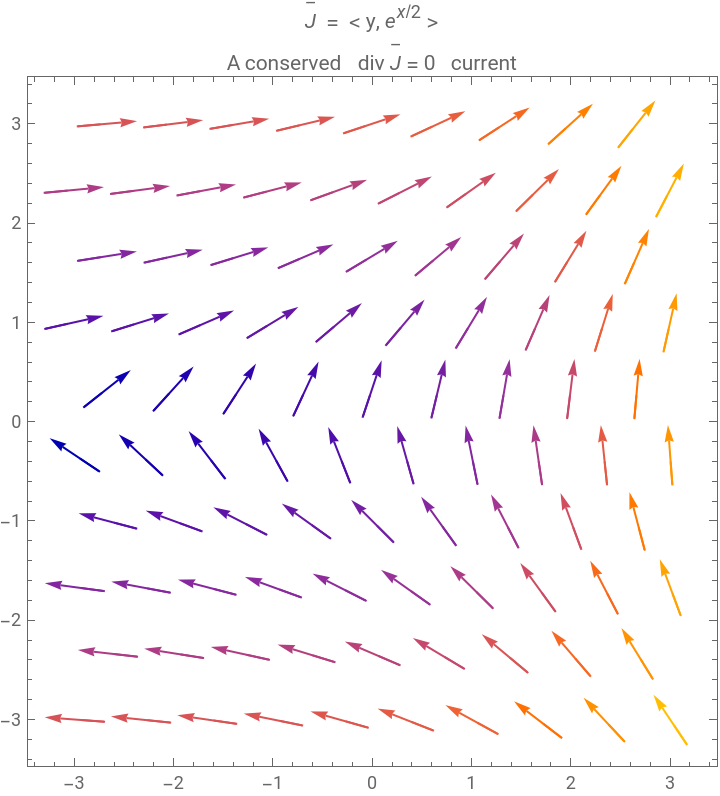
VectorPlot{y,Exp[x/2]},{x,-3,3},{y,-3,3},VectorPointsCoarse,VectorAspectRatio18,PlotLabel" = < y, >\nA conserved div = 0 current"
–
J
x/2
e
–
J
Out[]=
Setup
About the system
About the system
In this essay, I will explore a system described by the principle of least action, where action is an integral over an N-dimensional space with the integrand being a function of M scalar fields and their first derivatives.
S=∫L[,∇,,∇,...,∇]x
q
1
q
1
q
2
q
2
q
M
q
M
N
d
(
1
)q
1
q
1
q
2
q
2
Here the coordinates are Cartesian, x denotes the radius-vector, and x is the volume element. For example, the action could be given as , where u = u[t, x], v = v[t, x].
N
d
S=-uvdtdx
1
2
2
∂u
∂t
Notation I will be using
Notation I will be using
For the sake of shortness, I will be using the following conventions and notation:
◼
Einstein’s summation convention
◼
∂
i
∂q
∂
i
x
◼
·
q
dq
dt
◼
LL ≡ The Classical Theory of Fields, Landau and Lifshitz
Lemma 1
Statement
Statement
Lemma 1 states that
∂
j
J
∂
j
x
j
T
i
∂
i
s
∂
j
x
(
2
)Where is the canonical energy-momentum tensor of the system =-, s[x] is a vector field, and J is a vector field defined as follows.
T
j
T
i
∂L
∂
∂
j
q
k
∂
i
q
k
j
Lδ
i
j
J
j
T
i
i
s
(
3
)In particular, if =0, then the divergence of J is zero and hence, by Gauss’s theorem, its’ flux through any N - 1 -dimensional surface is zero, too.
j
T
i
∂
i
s
∂
j
x
Quite importantly, this lemma works not only if L is a function of scalar fields and their first derivatives, but also if L is a function of tensors of arbitrary rank and their first derivatives.
Short proof
Short proof
Original proof
Original proof
Energy-momentum conservation
Energy-momentum conservation
Lemma 2
Statement
Statement
Let us study the change of variables
x`=x+s[x]ε
(
6
)Where s[x] is a vector field and ε → 0.
Lemma 2 states that if the Lagrangian is invariant relative to this operation, then
∂L
∂
∂
j
q
k
∂
q
k
∂
i
x
∂
i
s
∂
j
x
(
7
)Proof
Proof
Theorem 1
Statement
Statement
If we find such vector field s that the Lagrangian is symmetric relative to the change of coordinates (6), and div s = 0, then J defined by (3) is a conserved current.
Proof
Proof
Finding conservation laws with the help of theorem 1
From the statement of theorem 1, it is clear that it can be used to find invariant quantities. This is the topic of this chapter.
Tools
Tools
The Algorithm
The Algorithm
Minkowski space and angular momentum
Minkowski space and angular momentum
Relation to Noether’s theorem
It is likely theorem 1 is a special case of Noether’s theorem, as both relate infinitesimal changes to conservation laws, but Noether’s theorem is more general. Although I haven’t been able to prove or disprove this statement, it is probably true.
As for the practical side, the Algorithm presented above has the same application as Noether’s theorem, namely - finding invariant quantities. However, the Algorithm is easier to use and is, arguably, more intuitive, although less general.
As for the practical side, the Algorithm presented above has the same application as Noether’s theorem, namely - finding invariant quantities. However, the Algorithm is easier to use and is, arguably, more intuitive, although less general.
Disadvantages in practical use
Disadvantages in practical use
Advantages in practical use
Advantages in practical use
Simplicity of use
Simplicity of use
To find a conserved current with Noether’s theorem, the researcher has to prove that the transformation of fields only changes the Lagrangian by a total derivative. This can be a fairly nontrivial problem, as I will show on the example below.
In the previous chapter, I’ve illustrated the use of the Algorithm on a particular system, where
S=∫LdtdxL=
4
∂u
∂t
∂v
∂x
In[]:=
exampleL
Out[]=
4
(0,1)
v
4
(1,0)
u
It can be seen that the Lagrangian is symmetric under the change of coordinates . In its’ infinitesimal version, it becomes t t + ε t, x x - ε x. Thus, s = < t, -x > .
tat,xx
1
a
Now that we know a symmetry, let’s try to find the corresponding conservation law.
Using Noether’s theorem
Using Noether’s theorem
Let us try to obtain the conservation law corresponding to s = < t, -x > using Noether’s theorem.
The change of coordinates
Is equivalent to the transformation of fields
The Lagrangian is then changed by
Now, to find the Noether’s current, we would have to find such F that
Which does not seem very easy. And as the Lagrangian gets more and more obscure, it becomes increasingly difficult to find F.
And even if F is relatively easy to find, it still requires human effort. The researcher has to carefully look at the expression for ∂L, possibly write it down in their notebook, and then spend time and brainpower trying to solve the problem.
Using the Algorithm
Using the Algorithm
Using the Algorithm, on the other hand, is incredibly simple. We just have to run the function tryS:
And we have the conserved current! Notice that the Lagrangian can be arbitrarily complex, because all the “dirty” work is done automatically.
So, as we have just seen, it is far easier to use the Algorithm than Noether’s theorem. This is because in order to find a Noether’s current the researcher has to manually solve a rather difficult problem of finding F, while in the case of the Algorithm most of the work is done by computer.
Intuition
Intuition
Easy to remember
Easy to remember
The Algorithm feels more intuitive than the Noether’s theorem, at least for me. This is because the formula (3) looks a lot like Noether’s theorem for particle mechanics. According to the latter, if the Lagrangian has the form
Now, compare it to (3):
The two latter equations are practically identical. The first factor on the right hand side of (3) is not momentum but the energy-momentum tensor, and the second term is not a single function but a vector field. However, the “essence” is very similar. And even though the way these two equations were derived is very different, the fact of their similarity might make memorizing (3) easier.
One more thing that makes (2) and (3) easy to remember is the fact that these formulas can be easily proven, as shown in the section “Lemma 1/Short proof”. After seeing it, the equations seem almost obvious.
In contrast, the statement of Noether’s theorem may not be as easy to remember, and the proof is relatively complex.
Intuitive formula for angular momentum
Intuitive formula for angular momentum
The expression for the density of the z-component of angular momentum derived with the Algorithm looks like this.
Notice how similar it is to the formula for angular momentum in Newton’s mechanics:
The formulas looks practically identical. This analogy helps to draw connections between field theory and Newton’s mechanics. If we used Noether’s theorem, this connection would not be so obvious.
Bibliography
Bibliography
◼
The Classical Theory of Fields, Landau and Lifshitz (abbreviated as LL)
CITE THIS NOTEBOOK
CITE THIS NOTEBOOK
An automatic procedure for finding conserved currents
by Rauan Kaldybaev
Wolfram Community, STAFF PICKS, September 25, 2020
https://community.wolfram.com/groups/-/m/t/2083630
by Rauan Kaldybaev
Wolfram Community, STAFF PICKS, September 25, 2020
https://community.wolfram.com/groups/-/m/t/2083630