KPZ equation
Numerically integrate=νf++ηwhere eta is Gaussian white noise
∂f
∂t
2
∂
∂
2
t
λ
2
2
∂f
∂x
In[]:=
sim[nu_,l_,dd_,dx_,nx_,dt_,nt_]:=Module[{f,nabla2,nabla,noise},nabla=SparseArray[{Band[{1,2}]->1.0,Band[{2,1}]->-1.0,{nx,1}->1.0,{1,nx}->-1.0},{nx,nx}]/(2dx);nabla2=SparseArray[{Band[{1,2}]->1.0,Band[{2,1}]->1.0,Band[{1,1}]->-2.0,{nx,1}->1.0,{1,nx}->1.0},{nx,nx}]/dx^2;noise:=RandomVariate[NormalDistribution[0,N@Sqrt[dd]],nx];NestList[Function[vec,vec+dt(nunabla2.vec+l/2(nabla.vec)^2+noise)],Table[0,{i,1,nx}],nt]];sim[nu_,l_,dd_,dx_,nx_,dt_,nt_,startvec_]:=Module[{f,nabla2,nabla,noise},nabla=SparseArray[{Band[{1,2}]->1.0,Band[{2,1}]->-1.0,{nx,1}->1.0,{1,nx}->-1.0},{nx,nx}]/(2dx);nabla2=SparseArray[{Band[{1,2}]->1.0,Band[{2,1}]->1.0,Band[{1,1}]->-2.0,{nx,1}->1.0,{1,nx}->1.0},{nx,nx}]/dx^2;noise:=RandomVariate[NormalDistribution[0,N@Sqrt[dd]],nx];NestList[Function[vec,vec+dt(nunabla2.vec+l/2(nabla.vec)^2+noise)],startvec,nt]];
Looks like a mess:
In[]:=
ListPlot3D[sim[1,1,1,0.1,100,0.001,100]]
Out[]=

First stromatolites:
In[]:=
maxsteps=60000;substeps=6000;plotstepsize=0.3;plotdata=sim[0.07,1,4.0,0.1,1000,0.001,maxsteps,Table[RandomReal[]+0.4Cos[i0.025],{i,1,1000}]][[substeps;;maxsteps;;substeps]]+Table[kplotstepsize,{k,1,maxsteps/substeps}];ListLinePlot[plotdata]
Out[]=
Nice earthy colors generated by Gemini 3 (rest of the code is my own)
In[]:=
(*Defineanchorcolors:DarkSlate,RawUmber,Olive,Sand*)anchors={RGBColor[0.25,0.25,0.25],(*DarkGrey*)RGBColor[0.4,0.3,0.2],(*DeepBrown*)RGBColor[0.55,0.5,0.35],(*OliveDrab*)RGBColor[0.7,0.65,0.55](*SiltyBeige*)};(*Generate20colorsbyblendingtheserandomlywithslightvariation*)stromatolitePalette=Table[Blend[anchors,RandomReal[](*Pickarandompointintheblend*)],{20}];(*Addalittlenoisetomakethemlook'unpolished'andnatural*)noisyPalette=(ColorConvert[#,"HSB"]&/@stromatolitePalette)/.Hue[h_,s_,b_]:>Hue[h+RandomReal[{-0.02,0.02}],Clip[s+RandomReal[{-0.05,0.05}],{0,1}],Clip[b+RandomReal[{-0.05,0.05}],{0,1}]];SwatchLegend[noisyPalette,Automatic,LegendLayout->"Row"]
Out[]=
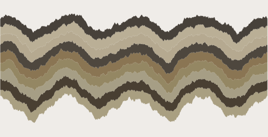
Combining it all into a nice Graphics object:
In[]:=
coords[i_]:=MapIndexed[{0.01#2[[1]],#1}&,plotdata[[i]]];polygons=Table[Polygon[Join[coords[i],Reverse[coords[i+1]]]],{i,Length[plotdata]-1}];Graphics[Riffle[Table[RandomChoice[noisyPalette],{i,1,Length[polygons]}],polygons],Background->Nest[Lighter,RandomChoice[noisyPalette],5],PlotRangePadding->{0,0.5}]
Out[]=