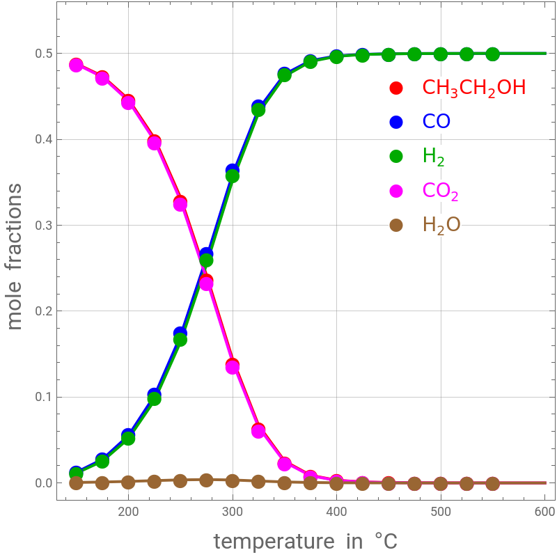
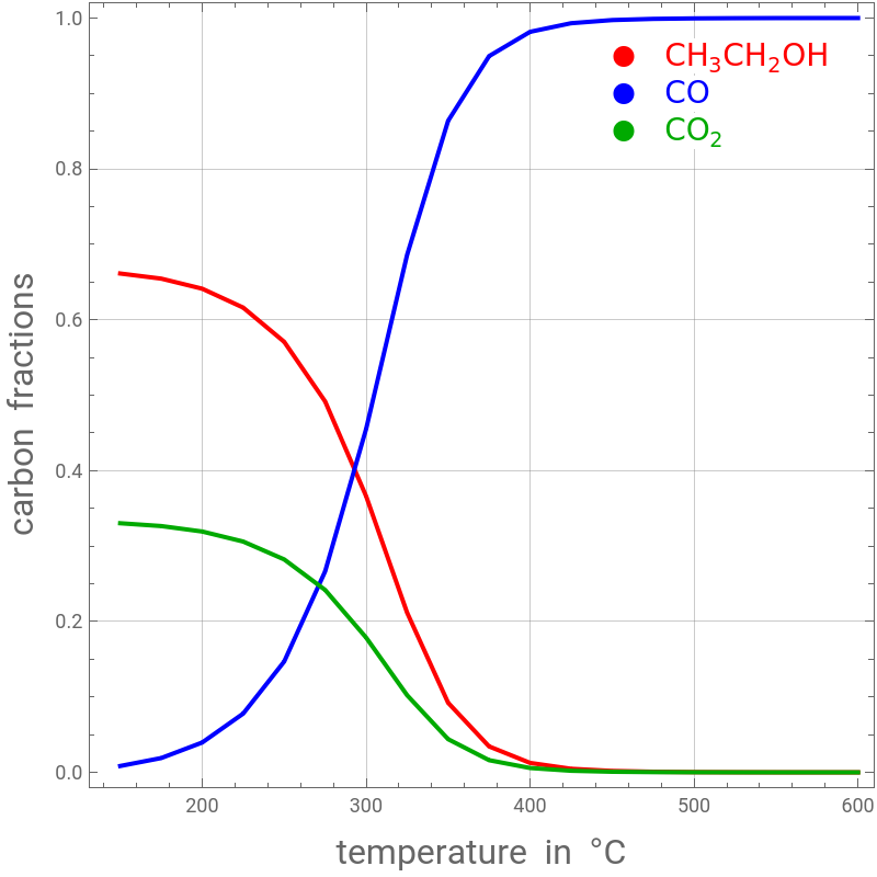
This notebook computes the thermodynamic equilibrium limits of converting syngas to ethanol by direct minimization of the total Gibbs free energy—the same physical approach used by Aspen Plus' s RGIBBS module—rather than by solving equilibrium - constant expressions . The system is a mixture of five species : CH₃CH₂OH (ethanol), CO, H₂ (syngas), CO₂, and H₂O, fed with a molar ratio H₂/CO = 1. Standard Gibbs energies of formation for each species are regressed against temperature from tabulated reference data, and the resulting fits are used to build the total Gibbs energy of the mixture, including the ideal - gas pressure correction . For each temperature and pressure, the equilibrium composition is found by minimizing this total Gibbs energy subject to non - negativity of all mole numbers and conservation of carbon, hydrogen, and oxygen atoms . Mole fractions and the derived carbon fractions (defined below) are computed and plotted versus temperature (25–2000 °C) at three pressures—1, 10, and 100 bar—each in its own section . At each pressure, the results are compared against reference values from Aspen Plus (using its built - in RGIBBS module, with Gibbs free energy minimization and the Peng–Robinson equation of state), and excellent agreement is observed throughout . Because the conversion of syngas to ethanol is highly exothermic and proceeds with a net decrease in moles (volume contraction), Le Chatelier' s principle predicts—and the results confirm—that high ethanol yields require low temperature and/or high pressure . Definition of the Carbon fractions: Let y₁, y₂, and y₄ denote the mole fractions of CH₃CH₂OH, CO, and CO₂, respectively . The carbon fractions are then= (for ethanol), = (for ), and = (for ).
C
1
2
y
1
2++
y
1
y
2
y
4
C
2
y
2
2++
y
1
y
2
y
4
CO
C
4
y
4
2++
y
1
y
2
y
4
CO2
In[]:=
Clear[P]
P = 1 atm
P = 1 atm
In[]:=
In[]:=
y[i_]:=n[i]/Sum[n[j],{j,1,5}];
In[]:=
Gtot[x_,P_]:=Re[Sum[n[j]*(G[x,P,j]+RxLog[n[j]/Sum[n[k],{k,1,5}]]),{j,1,5}]];G[x_,P_,1]:=((a1+a2x+a3x^2+a4x^3+a5x^4+a6x^5+a7x^6+a8x^7+a9x^8+a10xLog[x])/.solC2H6O)+RxLog[P/P1];G[x_,P_,2]:=((a1+a2x+a3x^2+a4x^3+a5x^4+a6x^5+a7x^6+a8x^7+a9x^8+a10xLog[x])/.solCO)+RxLog[P/P1];G[x_,P_,3]:=((a1+a2x+a3x^2+a4x^3+a5x^4+a6x^5+a7x^6+a8x^7+a9x^8+a10xLog[x])/.solH2)+RxLog[P/P1];G[x_,P_,4]:=((a1+a2x+a3x^2+a4x^3+a5x^4+a6x^5+a7x^6+a8x^7+a9x^8+a10xLog[x])/.solCO2)+RxLog[P/P1];G[x_,P_,5]:=((a1+a2x+a3x^2+a4x^3+a5x^4+a6x^5+a7x^6+a8x^7+a9x^8+a10xLog[x])/.solH2O)+RxLog[P/P1];
In[]:=
sol[T_,P_]:=Quiet@FindMinimum[{Gtot[T,P],Table[n[j]≥0,{j,1,5}],2n[1]+n[2]+n[4]1,n[1]+n[2]+2n[4]+n[5]1,6n[1]+2n[3]+2n[5]2},Table[{n[j],0.15},{j,1,5}],MaxIterations1000];as[T_]:=sol[T+273.15,P][[2]];
P = 1 atm
P = 1 atm
In[]:=
T=150;P=1;While[T≤600,{f=as[T],tbl1[T]=Table[{T,y[i]/.f},{i,1,5}],tbl2[T]={{T,2y[1]/(2y[1]+y[2]+y[4])/.f},{T,y[2]/(2y[1]+y[2]+y[4])/.f},{T,y[4]/(2y[1]+y[2]+y[4])/.f}},T=T+25}];data=Table[tbl1[T],{T,150,600,25}];data1=Transpose[data];p1=ListPlot[data1,JoinedTrue,PlotRange{-0.02,0.56},FrameTrue,GridLinesAutomatic,PlotStyle{{Red,Thick},{Blue,Thick},{Darker@Green,Thick},{Magenta,Thick},{Brown,Thick}},AspectRatio1,ImageSize400{1,1},FrameLabel{Style["temperature in °C",16],Style["mole fractions ",16]}];data2=Table[tbl2[T],{T,150,600,25}];p2=ListPlot[Transpose[data2],JoinedTrue,PlotRange{-0.02,1.02},PlotStyle{{Red,Thick},{Blue,Thick},{Darker@Green,Thick}},FrameTrue,GridLinesAutomatic,PlotStyleThick,AspectRatio1,ImageSize400{1,1},FrameLabel{Style["temperature in °C",16],Style["carbon fractions ",16]}];
In[]:=
Show[p1,pASPEN1,Graphics[{Style[Text["● OH",{450,0.46},{-1,0}],Red,14,BackgroundWhite],Style[Text["● CO",{450,0.42},{-1,0}],Blue,14,BackgroundWhite],Style[Text[Row[{"● ",}],{450,0.38},{-1,0}],Darker@Green,14,BackgroundWhite],Style[Text["● ",{450,0.34},{-1,0}],Magenta,14,BackgroundWhite],Style[Text[Row[{"● ",,"O"}],{450,0.30},{-1,0}],Brown,14,BackgroundWhite]}]]
CH
3
CH
2
Style["H",Plain]
2
CO
2
Style["H",Plain]
2
Out[]=
In[]:=
Show[p2,Graphics[{Style[Text["● OH",{450,0.95},{-1,0}],Red,14,BackgroundWhite],Style[Text["● CO",{450,0.90},{-1,0}],Blue,14,BackgroundWhite],Style[Text["● ",{450,0.85},{-1,0}],Darker@Green,14,BackgroundWhite]}]]
CH
3
CH
2
CO
2
Out[]=
P = 10 atm
P = 10 atm
In[]:=
T=150;P=10;While[T≤600,{f=as[T],tbl1[T]=Table[{T,y[i]/.f},{i,1,5}],tbl2[T]={{T,2y[1]/(2y[1]+y[2]+y[4])/.f},{T,y[2]/(2y[1]+y[2]+y[4])/.f},{T,y[4]/(2y[1]+y[2]+y[4])/.f}},T=T+25}];data=Table[tbl1[T],{T,150,600,25}];data1=Transpose[data];p1=ListPlot[data1,JoinedTrue,PlotRange{-0.02,0.56},FrameTrue,GridLinesAutomatic,PlotStyle{{Red,Thick},{Blue,Thick},{Darker@Green,Thick},{Magenta,Thick},{Brown,Thick}},AspectRatio1,ImageSize400{1,1},FrameLabel{Style["temperature in °C",16],Style["mole fractions ",16]}];Show[p1,pASPEN2,Graphics[{Style[Text["● OH",{450,0.42},{-1,0}],Red,14,BackgroundWhite],Style[Text["● CO",{450,0.38},{-1,0}],Blue,14,BackgroundWhite],Style[Text[Row[{"● ",}],{450,0.34},{-1,0}],Darker@Green,14,BackgroundWhite],Style[Text["● ",{450,0.30},{-1,0}],Magenta,14,BackgroundWhite],Style[Text[Row[{"● ",,"O"}],{450,0.26},{-1,0}],Brown,14,BackgroundWhite]}]]
CH
3
CH
2
Style["H",Plain]
2
CO
2
Style["H",Plain]
2
P = 100 atm
P = 100 atm