Recent discoveries have shown that well-known models of computation, such as cellular automata and Turing machines, can be “evolved” through random mutations of their instructions to create systems that are progressively more “fit” to achieve a certain goal, such as maximizing the lifetime that they run for before halting. This project aims to take this phenomenon and try to understand it from a new lens by applying it to another model of computation: the register machine. A register machine can be thought of as a simplified representation of the modern-day CPU (Central Processing Unit) found in smartphones, laptops, and various other devices. CPUs often contain many registers (and many different types of instructions), but simple register machines are usually made up of just two registers, with each holding a non-negative integer value; these registers are updated as an accompanying set of instructions is processed, with each instruction being one of two typical operations: an increment or a decrement-jump. In this project, a simple and highly customizable register machine is first developed and then evolved under various conditions, and its behavior is analyzed. Ultimately, this project aims to provide the grounds for which future researchers can experiment with random (weighted) growth from a simple, highly customizable program and perform a deep dive into the phenomenon of complex behavior arising from simple processes through the lens of a model that behaves differently from cellular automata or Turing machines.
Initialization
Initialization
Introduction to Computational Models
Introduction to Computational Models
Cellular Automata
Cellular Automata
Introduction to Cellular Automata
Introduction to Cellular Automata
A well-known model of computation with simple instructions that can display complex behavior is a cellular automaton. Cellular automata programs are composed of cells, with each cell holding a value representing its state (usually simply “on” or “off”) and possessing an understanding of its “neighborhood.” In the case of 1-dimensional CA, this usually means that, for each cell, you will need to look at 3 cells: the current cell, the cell to its left, and the cell to its right; the size of the neighborhood can change based on the radius one chooses to observe. A common way that the rules of a CA are visualized is shown below.
In[]:=
RulePlot[CellularAutomaton[30]]
Out[]=
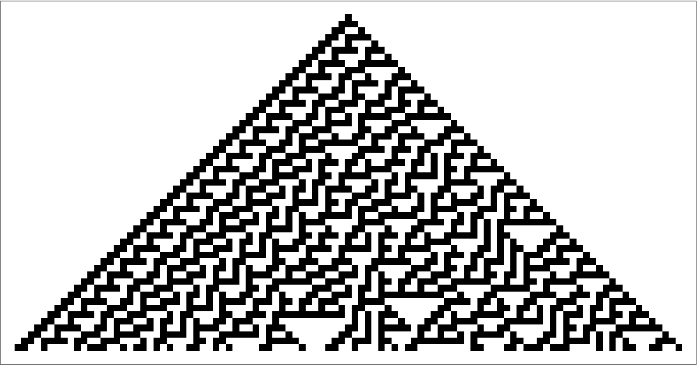
Here, the CA is made up of 8 rules because there are 8 possible scenarios when observing the neighborhood. For each rule, the cell currently being looked at is at the top of the visual in the middle and its neighbors (including itself in the center) are at the top of the visual. The second rule in the set above, for example, is saying that if the cell’s two left neighbors are “on” and its third neighbor is “off”, then the current cell should be set to “off”. A simple set of rules like the one above can be simulated and lead to very complex output, like so:
In[]:=
Column[{ArrayPlot[CellularAutomaton[30,{{1},0},50],ImageSize->500],"Rule 30"},Alignment->Center]
Out[]=
Rule 30 |
Adaptive Cellular Automata
Adaptive Cellular Automata
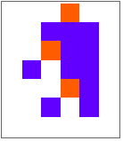
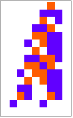
In December 2024, Stephen Wolfram, Richard Assar, and Nik Murzin made an interesting discovery regarding these cellular automata: these simple programs can be treated as lifeforms by evolving them to get better and better at a certain goal using purely random mutations and deterministic selection of these mutations. The process would be to start with an initial ruleset and play it out until it came to a full halt (a fully empty row). The number of rows would be described as the “height” or “lifetime” of the automaton. Then, a random, single-point mutation will be made, meaning that one single rule will be changed such that the automaton exhibits different behavior when run again. If this mutation leads to a longer “lifetime,” the mutation is kept and used as the basis for future mutations so that the lifeform can only keep improving, or “evolving.” Mutations that do not lead to better lifetimes are discarded. Perhaps the most important discovery in this system was the importance of intermediate steps. By holding onto not only mutations that lead to longer lifetimes but also so-called “lateral mutations” that lead to the same lifetime, more possibilities are opened up and the lifeforms are therefore given a wider range on which they can evolve. These adaptive cellular automata (CA) can be run in Wolfram Language, as seen below.
A “breakthrough” is defined as a rule that leads to a new maximum fitness. Breakthroughs do not include lateral mutations.
Running an adaptive CA program that plots the “breakthroughs” for a system that evolves 500 times
In[]:=
SeedRandom[100];ResourceFunction["AdaptiveCellularAutomaton"][<|"AdaptiveIterations"->500|>,"BreakthroughStates","Plot"]
Out[]=
,

,

,

,
,

Register Machines
Register Machines
In Stephen Wolfram’s A New Kind of Science, register machines are described as being “specifically designed to be very simple idealizations of present-day computers” (Wolfram 97). Most modern computers have many registers, and each register’s value is able to be changed by various kinds of instructions; register machines are a way of modelling these CPUs on a small scale by having a small amount of registers that are changed by a small variety of instructions. In most simple register machines, there are 2 registers, with register 1 depicted as being light gray and register 2 as being dark gray. In the program, however, the user has the ability to specify how many registers they want the program to have. Each of the registers can follow one of three instructions, with two of them being traditional, simple instructions and one being an extra added in for the potential of added complexity:
◼
Increment, which increments the value stored in the register by 1 (traditional)
◼
Decrement-jump, which skips to the next instruction if the register holds a value of zero and otherwise decrements the value held by the register by 1 and jumps to the step specified by the instruction (traditional)
◼
Skip, which skips over the instruction entirely (unique to my machines)
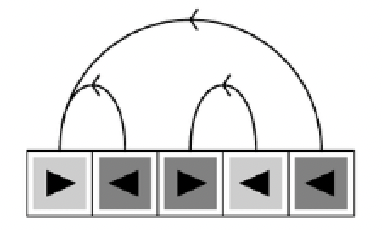
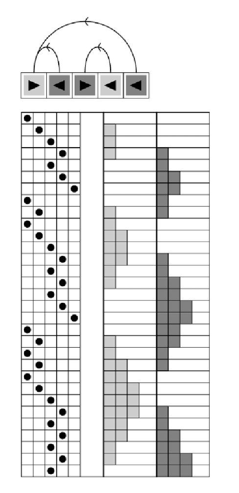
The visualization below shows an example sequence of instructions, with right-facing arrows representing increments and left-facing arrows representing decrements. In this example, the first step is an increment to the first register, the second step is a decrement to register 2 with a jump to step 1, the third step is an increment to register 2, the fourth step is a decrement to register 1 with a jump to step 3, and the fifth step is a decrement to register 2 with a jump to step 1.
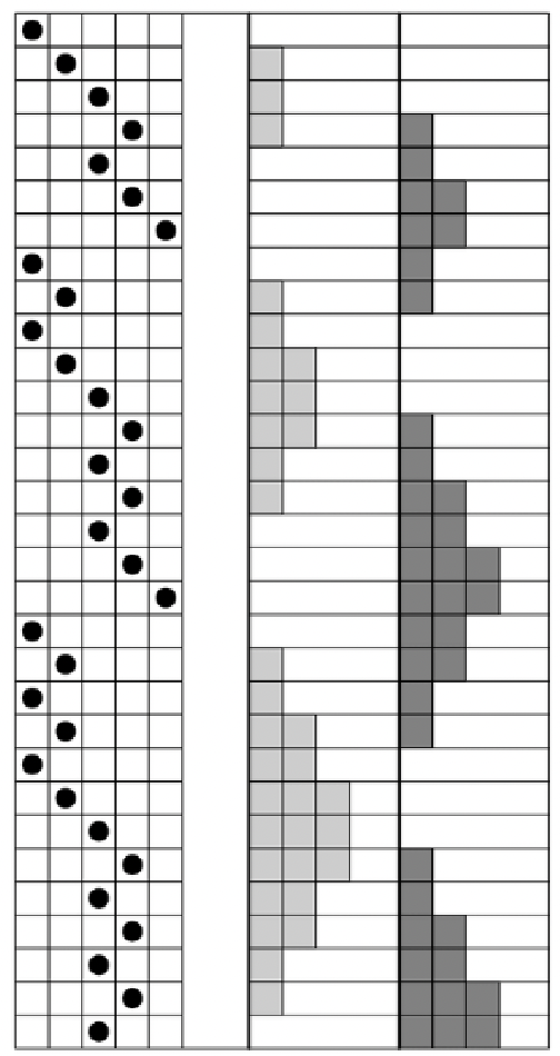
The diagram below is split into rows, and each row corresponds to a step in the computational program, with the dots on the left indicating the instruction being evaluated on a given step. To the right of the step visualizer is a graphic of the values of each register after each step, with each row representing the register values at that moment in the sequence of the execution of instructions. In the example below, both registers (the two columns on the right) start at a value of zero. After instruction 1 is run, looking at the second row, one can see how register 1 has one block inside of it, which corresponds to a value of one and indicates that register 1 has a value of 1 after the previous step had been run. This continues for the rest of the sequence (which could be infinite).
Throughout the project, for cases with low fitness values, a combination of the top two visuals is used as a way of expressing the data in a visually appealing way that also adheres to the literature from which it came. Below is an example of what this could look like.
The idea of taking a computational model that follows simple, defined rules and mutating these rules to produce complex behavior is not limited to cellular automata. In fact, any machine that strictly adheres to a set of rules can be adapted through modifications of these rules. Turing machines are great examples of this. This project aims to further this phenomenon by applying the ideas of adaptive cellular automata to register machines, a simple program that follows rules slightly differently than cellular automata and Turing machines do. Instead of having a set of all possible cases and simply matching each situation in the machine to a case, register machines execute sets of instructions and update the corresponding register after each step. A halting point in a Turing machine happens when a certain pattern triggers the case that ends in a halt instruction, and a halting point in cellular automata happens when an entire row of “off” cells is generated, which leads to the rule of an empty neighborhood being triggered for an infinite number of times. Halting points in register machines, on the other hand, happen when a register machine successfully executes the last step in the linear sequence and does not jump back to anywhere else in the program. Because of these differences between cellular automata/Turing machines and register machines, I went into this project with an understanding that my results may lead to wildly different behavior than the behavior typical of adaptive Turing machines and adaptive cellular automata.
Before beginning my project, there was one key issue that needed to be addressed: it is not uncommon for Turing machines and cellular automata to halt, especially when dealing with random rules and starting from a null set of rules. Register machines, on the other hand, are much, much more likely to continue forever than to halt, despite their “linear” nature; this behavior can be attributed to the existence of decrement-jumps, which can send the program backwards and often create infinite loops. To address this issue, a metric would need to be established to measure fitness other than purely lifetime, because then most register machines would have the same pure lifetime of Infinity (or whatever value is specified by ). As a solution, fitness is to be measured like so: specify a register for the program to track and a value to look out for. The program first tests for validity by checking whether the specified value is reached by the specified register within . If it does not, the mutation is immediately discarded. If it does, a second check is run that tests the “fitness” of the mutated register machine, which is defined as the number of steps before the specified register reaches the target value and “overflows.” The system’s fitness goal is to drag the process out for as long as possible before the specified register reaches the specified value. With these considerations in mind, it was time to begin building the model.
MaxSteps
MaxSteps
Approach
Approach
Simulating a simple register machine
Simulating a simple register machine
Simulating a single instruction
Simulating a single instruction
The very first step in the project was to develop a way to simulate a register machine that executed a defined set of instructions. This instruction set can be represented as a nested list, with the length of the outer list being the number of instructions and each element of the outer list representing an instruction and holding the necessary info about how to execute it. The structure of the list representing a single instruction is as follows:
◼
The first index indicates the number of the register the instruction acts upon (each register is identified by its number: 1, 2, ...)
◼
The second index specifies the type of instruction with a numerical value: 1 for increment, 0 for skip, and -1 for decrement
◼
The third index tells what step in the program a decrement-jump block will jump to. This value is either 0 (for increments or skips) or a number representing the position in the list to jump to. Note that jumps can be forwards or backwards
◼
The fourth index stores the index of the instruction relative to the whole instruction set. For example, the eighth element in the outer list would have 8 as its fourth index
Numerical representation of the ruleset shown in the Introduction:
In[]:=
basicInstructions={{1,1,0,1},{2,-1,1,2},{2,1,0,3},{1,-1,3,4},{2,-1,1,5}};
We can use the helper function to reformat the data. The main difference between the original list and the new list returned by has to do with the fact that the new list holds the values of the registers after each step alongside the relevant instruction information for that step, combining two separate parts of the machine into one list. The registers in a register machine are considered separate from the instructions of the machine because although the instructions are executed on the registers, the same is not true for the other direction; the registers have no way of interacting with the instructions. Using , a basic instructions list can be converted into the necessary data to nestedly execute the instructions of the register machine. The function takes the argument of to represent the initial values of each register (usually all 0) and as the set of instructions to be carried out.
buildList
buildList
buildList
buildList
regVals
ruleSet
Defining the helper function to build a list containing the values of each register as well as other data that allows the computer to understand the nature of the current instruction:
In[]:=
ClearAll[buildList];buildList[regVals_,ruleSet_]:={regVals,ruleSet[[1,1]],ruleSet[[1,2]],ruleSet[[1,3]],2}
The function outputs a list where:
buildList
◼
Index 1 is a list of the values held by each register at the step immediately before
◼
Index 2 is the number of the register currently being acted on
◼
Index 3 is the current instruction type (increment, skip, or decrement)
◼
Index 4 is the instruction to jump to (0 if the step isn’t a decrement)
◼
Index 5 is the index of the next step that will be carried out
All of the information in this list will later be fed into a nesting function that updates each value until the end of the instruction set is reached, the program has hit the maximum number of steps, or the program encounters “overflow.”
Converting the instruction set from the input format to the format expected by the program, with a starting value of 0 for all registers:
Update the state of the program by moving on to the next instruction in the sequence:
Execute a single instruction of an instructions set:
Simulation of executing the first few instructions in the basic instruction set, keeping track of whether register 1 reaches a value of 2:
For comparison, observe how the output would look without the checks in place.
Simulating a set of instructions
Simulating a set of instructions
Defining the function to simulate the entire process of running through the ruleset of a register machine:
The function also works for instruction sets that come to a halt, in which case the program will terminate early
Visualizing the Register Machine
Visualizing the Register Machine
Function to generate a visualization of the instructions for any register machine program:
Example of the function, using a side-by-side comparison with the basic instruction set for the simplified view and the full view:
This helper function creates one row in the visualization of every step of the instruction sequence:
This function builds the grid that has the step number as the row number and the instruction number as the column number:
Visualize the steps in a more time- and resource-efficient way:
This function is used to show the value of a specified register at a single step:
This function allows us to see the value of the registers at each step through the sequence of rules:
Visualize the basic data for each register:
Just as I did for the step tracker, I can create a simplified and less Graphics-intensive way of visualizing the register machine values by using a line plot
This function allows us to see the value of the registers in an efficient way:
Putting all the visuals together, with adjustments made based on the desired view type:
Example of a full visualization of the past data in all 3 view types:
Adaptive Register Machine
Adaptive Register Machine
Now that I have a working and easily understandable register machine, I can begin the process of mutating rules in the register machine and observing changes across iterations. I will be performing single-point mutations, meaning only one change is made each iteration, allowing us to more easily identify what specific factors lead to the growth of a system. The way the computer decides on the type of mutation is random, but the weighted probabilities of the different mutations can be adjusted. The tree diagram below shows the hierarchy of mutation types and how the computer chooses each one. Note that percentage values that aren’t bolded are dependent on the characteristics of the instructions and not on weights.
◼
The bolded numbers are dependent on user-defined weights
◼
The unbolded percentages are based on the set of instructions
◼
In the diagram below, the unbolded percentages were computed from the instruction set defined to the left of the figure
In the program, create an association of weights representing the relative weighted probability of each event happening to model the bolded probabilities in the decision tree above.
Association mapping keys (outcomes) to their values (relative weights). These weights all have the same values as those in the flowchart.
I then build up the rule mutation function piece-by-piece. I begin by picking a random step from the instructions list and identifying the position of this step.
Pick a random step from the basic instructions and identify its position:
I can split the decision tree into its component branches:
Run when a skip instruction is selected
Run when an increment/decrement instruction transforms into a skip instruction
Run when an increment instruction is selected
Run when a decrement instruction is selected
Run when a non-skip instruction is selected
Run when a non-skip instruction is to be evaluated
Code representing the different possible outcomes from the decision tree flowchart:
Helper function to choose a random position to put an arrow at as a way of mutating the register machine:
Helper function to change the register that an increment/decrement step is performed on:
Putting it all together in one giant mutation function:
Example of a mutation:
Putting it all together
Putting it all together
Defining the program function, which puts all of the code together for a single register machine:
Example of running the full register program on the previous instruction set, with a maximum steps of 40, a non-simplified view, a return of all the values of register 2, and three registers all set to 0:
All the customization options for the finalized adaptive register machine function:
Defining the structure and parameters of the function:
Running the initial register machine, using the default values of the basic instructions, three registers starting at 0, 40 steps max, and keeping track of when register 1 hits a value of 6:
The register machine now adapts and shows a timeline of mutations and their effects on the register of interest:
Adding on to the code to filter out instructions that deteriorate fitness:
The main function now allows us to better understand the data at each step:
Perform necessary operations when a mutation is accepted
Finalized adaptive register machine function:
Running an adaptive register machine with a new set of instructions
Data Visualization
Data Visualization
Nicely display the rule evolution of the adaptive register machine:
Function definition for the progressive maximum fitness alongside a graph of all fitness values:
Plot the edit distance of each mutated ruleset from the original ruleset:
Easily view all important data:
Experiments & Results
Experiments & Results
Store the various rule sets to use for the experiment
Generate a list that, for each register machine created by a ruleset from the instruction set, creates a line plot of the best fitness across iterations alongside a scatter plot of the fitness value of each attempted mutation. The returned list is the line plot, followed by the number of instructions, followed by the best recorded fitness overall.
Run the rulesets across various random seeds for more reliable data by returning an association of key-value pairs for each new random seed. Each key-value pair goes NumInstructions -> BestFitness. Thus, each association has 98 key-value pairs.
Finally, I can average these values by creating a table that runs from 3 to the length of each association + 2 (100) and averages the values from each different random seed. I then put this into a ListLinePlot to visualize the average output. Here, the x-axis represents the number of rules in the ruleset and the y-axis represents the highest fitness achieved.
Line plot showing the average highest fitness value achieved for different instruction set lengths:
One can see from the results that in the early stages there is a very noticeable and direct relationship between the number of instructions and the maximum fitness achieved by that instruction set. In the middle we see a consistently high maximum fitness, which is interesting and could perhaps be the case because there is just the right balance between having too many instructions such that changes are too small and thus many iterations are necessary for growth and having too few instructions such that changes are very hit-or-miss and can lead to massive improvements but happen very, very infrequently. With that said, I still see very high maximum fitness values being achieved in the later stages, but none reach the peak achieved by the ruleset with 51 rules. Even the second-highest value, of 237.9, only lies in the set with 49 rules. Another trend is that the amplitude of the graph (difference between relative highs and lows) seems to be getting smaller and smaller as the number of instructions increases. For example, the distance from x = 40 to x = 51 is 137.9, while the distance from x = 76 to x = 84 is only 110.4, and the distance from x = 94 to x = 99 is a mere 65.9.
Here, we observe an interesting contradiction to a belief held prior to the experiment. Previously, it was believed that adjusting the selection function to allow for lower fitness values would lead to the machine being able to branch more and thus find higher fitness values, but it turns out that for every single case in this experiment, the register machines performed more poorly with the new selection function than they did with their original selection function. For example, in the very last situation, the best random seed only peaked at a value of around 330, while in the original 2 different random seeds were able to make it over 330 fitness and other seeds also generally performed better than they did with the modified selection function.
The next experiment investigates the effect of removing “skip” instructions from the mutation decision tree by setting its weight value to 0.
Here, we see that having skips generally leads to higher fitness values, thus highlighting their importance even though they may be seen as useless, “empty” blocks. The next experiment is similar to the last one but instead adjusts the weights to remove register flipping operations for instructions.
Here we see that getting rid of register changes is also bad for our maximum fitness. We then finish the experiments by investigating the effect of adding more registers to the machine and observing the effect on fitness and mutation distance.
One can see here that, as the overflow values increases, the slope of the function becomes significantly less steep, demonstrating an interesting relationship between overflow value and the maximum fitness since, after a certain point, the overflow value seems to stop having an effect on the maximum fitness being reached by the system. Perhaps a different metric takes over and becomes a greater influence on the behavior of the register machine, or perhaps at such high overflow values register machines are unable or very, very unlikely to break past a certain threshold that leads to improved behavior.
Conclusions
Conclusions
Reflecting on the process of building the skeleton for the register machine, it can be seen as a relatively straightforward (though still time-consuming) process and can be very easy to interpret. It follows a defined set of rules and produces the same output every single time. Values can be changed, such as the instruction set or initial register values, but these lead to entirely different register machines being created. With adaptive register machines, I introduce a resemblance of ancestry where successive register machine generations (evolutions) have genotypes similar to their parent machine and may exhibit similar behavior (or the exact same behavior, despite a changed rule) or may exhibit wildly different behavior, highlighting the unpredictability of evolution. On that note of unpredictability, adaptive register machines are fascinating in their random natures, and having the ability to run the same line of code that starts with the same register machine and watching it evolve in vastly different ways each time feels as though I am watching different timelines unfold and seeing how small changes can drastically alter systems for better or worse. The uncertainty associated with these computational models is almost unbelievable at times, cementing register machines as more than computational models, but instead tools for analyzing lifelike systems from a computational lens.
Future Directions
Future Directions
Trivial Modifications
Trivial Modifications
Data Analysis
Data Analysis
Adaptive Fractal Systems
Adaptive Fractal Systems
Another future direction is much more general, and that is to continue exploring the concept of simple machines adapting and evolving to meet a certain goal by investigating this behavior in other simple machines. Stephen Wolfram’s book A New Kind of Science describes in detail many different kinds of programs and thus would be a good place to find inspiration for the next adaptive machine. One particular machine that I think would be interesting to implement would be a two-dimensional substitution system, which works similar to cellular automata by looking at the value of a cell and having a rule tell the program what to do based on that value. Two-dimensional substitution systems do not care about neighborhoods in the way that CA does. Below is from page 187 of A New Kind of Science and shows the evolution of a 2D substitution system. The rules can be observed in the bottom left.
I believe that 2D substitution systems with evolution could be very interesting because without evolution the machine already generates very interesting visuals and with evolution one can only imagine what sorts of patterns and randomness could arise from these systems. 2D substitution systems also provide more mutation choices. For example, changing a rule as a mutation could look like changing a single square in the resulting grid instead of merely changing the value from “on” to “off” or vice-versa as is the case with CA. Fitness functions would be difficult with this system due to its nested behavior, but a potential fitness function could be measuring consecutive white tiles that aren’t padding tiles (i.e. white tiles inside the main shape). Perhaps I want to maximize the time before 20 consecutive white tiles appear within the main shape. Consecutive could also mean horizontally, vertically, or even diagonally, allowing for lots of customization.
More ways of visualizing data
More ways of visualizing data
A future direction that I find to be very interesting is exploring other ways to visualize the data beyond simple line plots and bar graphs. This future direction was inspired by page 100 of A New Kind of Science, where Wolfram first shows the everyday Full view register machine for an 8 instruction machine:
He then shows a compressed version of the evolution that only shows the steps where either register has just decreased to zero and the other’s value is displayed:
Then, the values held by register 2 at steps where the first register has just decreased to zero (all the numbers in the second register column above) are converted to binary digit sequences and plotted, with blacks representing 1s and grays representing 0s.
The result is a pattern reminiscent of a cellular automaton through this approach despite the very different natures of the two machines. Perhaps by adding in evolution, I could generate some very interesting patterns that exhibit some sort of complex behavior.
Further investigating the fitness and selection functions
Further investigating the fitness and selection functions
A final question to consider is whether evolution searches for complexity at all. According to Stephen Wolfram, there are 11,019,960,576 possible register machines with a length of eight instructions, and of that number only 126 exhibit what can be classified as complex behavior (non-repeating, non-nested, randomness, etc). When performing evolutions, is this complex behavior preferred over other behaviors? Does evolution search for greater complexity? Or does complexity not matter in the grand scheme of things if all I care about is maximizing a certain goal? What does this say about biological evolution?
References
References
◼
Wolfram Function Repository. (n.d.). AdaptiveCellularAutomaton. https://resources.wolframcloud.com/FunctionRepository/resources/AdaptiveCellularAutomaton
◼
Wolfram Function Repository. (n.d.). AdaptiveTuringMachine. https://resources.wolframcloud.com/FunctionRepository/resources/AdaptiveTuringMachine
◼
Wolfram, S. (2002). A new kind of science. Wolfram Media. https://www.wolframscience.com/nks/
◼
Wolfram, Stephen. “Foundations of Biological Evolution: More Results & More Surprises.” Stephen Wolfram Writings, Dec. 2024. writings.stephenwolfram.com, https://writings.stephenwolfram.com/2024/12/foundations-of-biological-evolution-more-results-more-surprises/
◼
State evolution in multiway register machines featuring applications to recursive functions --Wolfram Community. (2025). STAFF PICKS. https://community.wolfram.com/groups/-/m/t/3499350
Acknowledgements
Acknowledgements
I would like to acknowledge my mentor, Nicholas Frieler, for using his expertise with adaptive Turing machines to guide me through a project in an area of study (adaptive simple machines) that has sparse literature and can be difficult to establish a clear direction in. Alongside helping me fix syntax errors in my code and polish my essay, he gave me clear guidance throughout the project (and adjusted the project direction whenever necessary) that allowed for great progress to be made each day and allowed the work from each day to nicely build on itself and result in the project as it is today. I would also like to acknowledge all of the teaching assistants (TAs) who helped me throughout my project, specifically Bryan Chen for making the entire program a truly enjoyable experience and serving as an example for balancing work and play. Additionally, I would like to acknowledge Rory, Eryn, Megan, and Cyrus for maintaining such an incredible and unique program.
Additional thanks to Stephen Wolfram for suggesting this project.
Additional thanks to Stephen Wolfram for suggesting this project.
CITE THIS NOTEBOOK
CITE THIS NOTEBOOK
Modeling and exploring adaptive evolution with register machines
by Mason Pinkerton
Wolfram Community, STAFF PICKS, July 9, 2026
https://community.wolfram.com/groups/-/m/t/3754313
by Mason Pinkerton
Wolfram Community, STAFF PICKS, July 9, 2026
https://community.wolfram.com/groups/-/m/t/3754313